Week 3 Practice: Data Wrangling & First Tableau Charts
BUS220 - Business Intelligence and Analytics
Submission Checklist
2 points (satisfactory completion) | Deadline: 3 days after the practice session
Submit three files in Moodle:
File 1 — billboard-long.csv (Session 1, Parts 1-4):
File 2 — billboard-songs.csv (Session 1, Part 5):
File 3 — Tableau workbook (Session 2):
Tools & Data
Session 1 instructions use Syto (syto.app) — browser-based, no install needed. If you prefer Python, R, or another tool, the expected outputs are described at each checkpoint. The steps are the same conceptually; you’re on your own for tool-specific details.
Session 2 uses Tableau Public — download from public.tableau.com.
Dataset: billboard-raw.csv — download from Moodle.
Billboard Hot 100 chart data from 2000: 317 songs with weekly rankings across 76 week columns (x1st.week through x76th.week). The problem: “week” is a variable, not 76 separate variables. Your job is to fix this.
Session 1: Data Wrangling
Part 1: Import & Inspect
- Import
billboard-raw.csvinto Syto - You should see 317 rows, 79 columns
- Scroll right to see the 76 week columns — most cells are empty
Part 2: Reshape
Remove unnecessary columns
Columns tab > Edit columns. Remove year and date.peaked — they add no information.
Unpivot
Table tab > Unpivot. Choose “Columns to keep (as index)” and select the metadata columns: artist.inverted, track, time, genre, date.entered. The 76 week columns become key-value pairs. Name the key column week_label and the value column rank.
You should now have roughly 24,000 rows — 317 songs x 76 weeks, with many empty ranks.
Filter out missing ranks
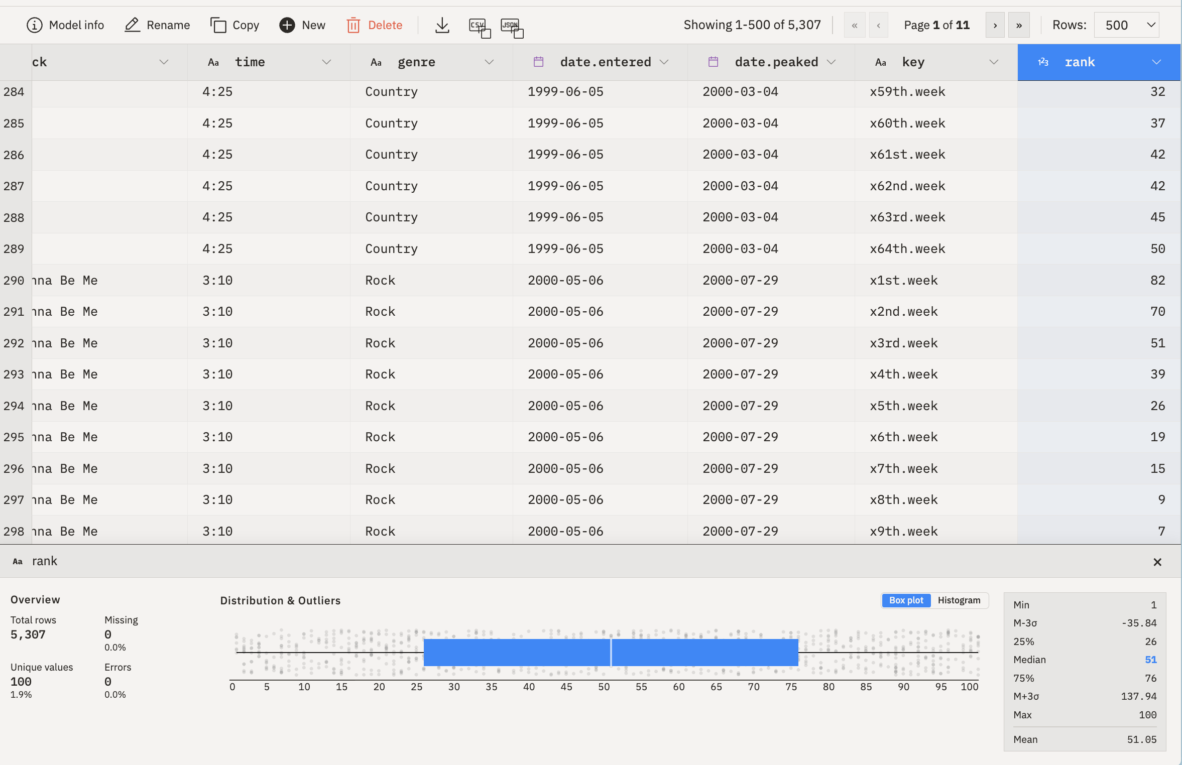
Rows tab > Filter. You need to remove rows where rank is null or an empty string (the raw data has both). Try: rank != null && rank != ""
After filtering, you should have exactly 5,307 rows. If you have 24,000+, the filter didn’t work. If you have slightly more than 5,307, empty strings survived — check for blank values in the rank column.
Part 3: Clean & Derive
Rename columns
Columns tab > Edit columns:
artist.inverted>artistdate.entered>date_entered
Extract week number
The week_label column has values like x1st.week, x22nd.week. You need just the number.
Columns tab > Extract. Source: week_label, regex: (\d+), capture group: 1, new column name: week. Then remove the original week_label via Edit columns.
Fix data types
Columns tab > Convert:
week> Integerrank> Integer (check “Strip non-numeric characters first”)date_entered> Date
Derive duration_seconds
The time column has values like 3:33 (minutes:seconds). Create a numeric column duration_seconds by splitting on : and computing minutes * 60 + seconds.
Columns tab > Derive. Name: duration_seconds. You’ll need to extract the minute and second parts and combine them — try Syto’s string and math functions in the expression editor.
Derive chart_date
The calendar date of each ranking: chart_date = date_entered + (week - 1) * 7 days.
Columns tab > Derive. Name: chart_date. Use Syto’s date arithmetic functions — the expression editor has autocomplete.
If you can’t get chart_date working, skip it. You can create it later in Tableau: DATEADD('week', [Week]-1, [Date Entered]).
Part 4: Validate & Export
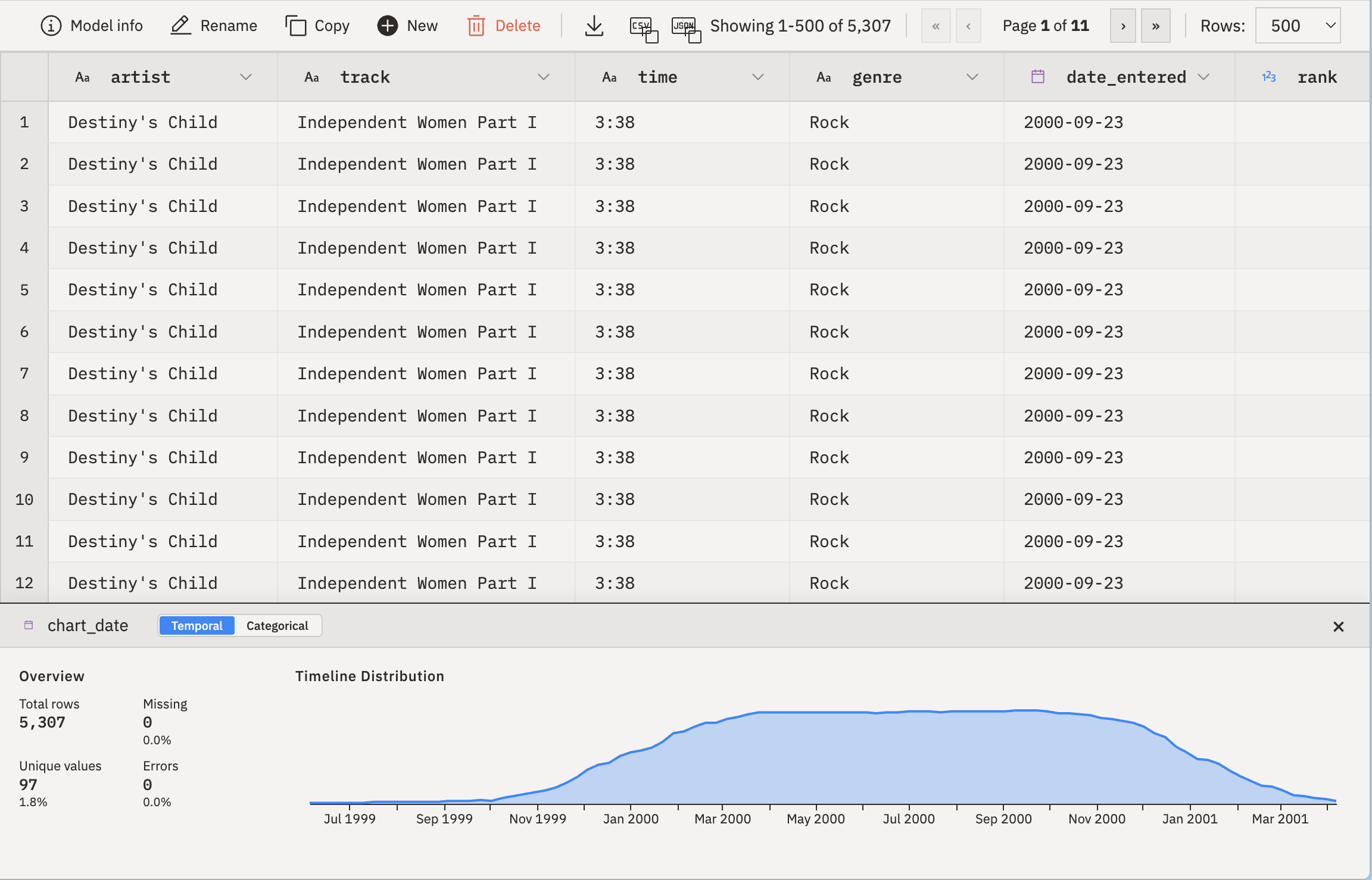
- 5,307 rows, 8-9 columns
- Columns:
artist,track,time,duration_seconds,genre,date_entered,week,rank,chart_date weekandrankare integers, dates are dates, no nulls inrank
Export as CSV: billboard-long.csv
Part 5: Song-Level Summary
Group your long data to one row per song.
Table tab > Group by:
- Group by:
artist,track,time,genre - Aggregations:
weeks_on_chart= count of rowspeak_rank= min ofrank(rank 1 is the best)
Optionally, add a songs_by_artist column: count how many unique songs each artist has. This is a window calculation — after grouping, count rows per artist and assign that number back to every song by that artist. In Syto, try using Derive with a window/partition expression after the group-by step.
- ~316 rows, one per song
weeks_on_chartranges from 1 to ~57peak_rankranges from 1 to ~99
Export as CSV: billboard-songs.csv
Session 2: First Steps in Tableau
If you didn’t finish Session 1, download the pre-built CSV files from Moodle.
Part 1: Connect Data
- Open Tableau Public
- Connect > Text file > select
billboard-long.csv - Verify types: dates show calendar icons,
rank/weekshow#, text fields showAbc - Click Sheet 1 to go to a worksheet
- Add the second data source: Data > New Data Source > connect
billboard-songs.csv
You can switch between data sources using the Data Source selector in the toolbar.
rank is numeric, so Tableau defaults to SUM — but summing ranks is meaningless. When using rank, change the aggregation to MIN, AVG, or MEDIAN.
Part 2: Guided Worksheets
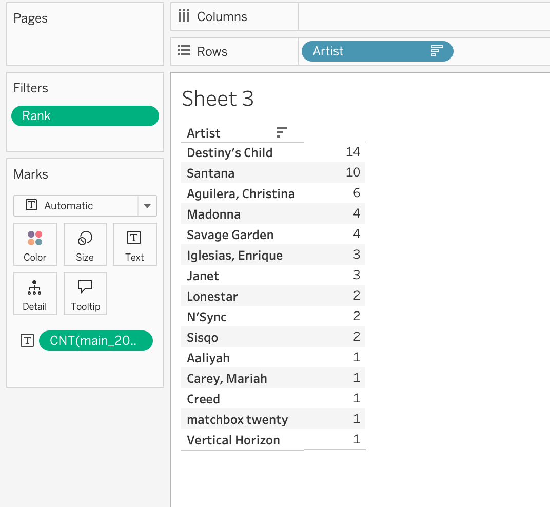
Worksheet 1: Artists with Most Weeks at #1 (bar chart)
Data source: billboard-long.csv
- Drag
artistto Rows - Drag
rankto Filters — filter to only rank 1 - Drag
chart_dateto Columns — change the aggregation to CNTD (count distinct) to count the number of weeks at #1 - Sort descending (toolbar sort icon)
- Title: “Artists with Most Weeks at #1”
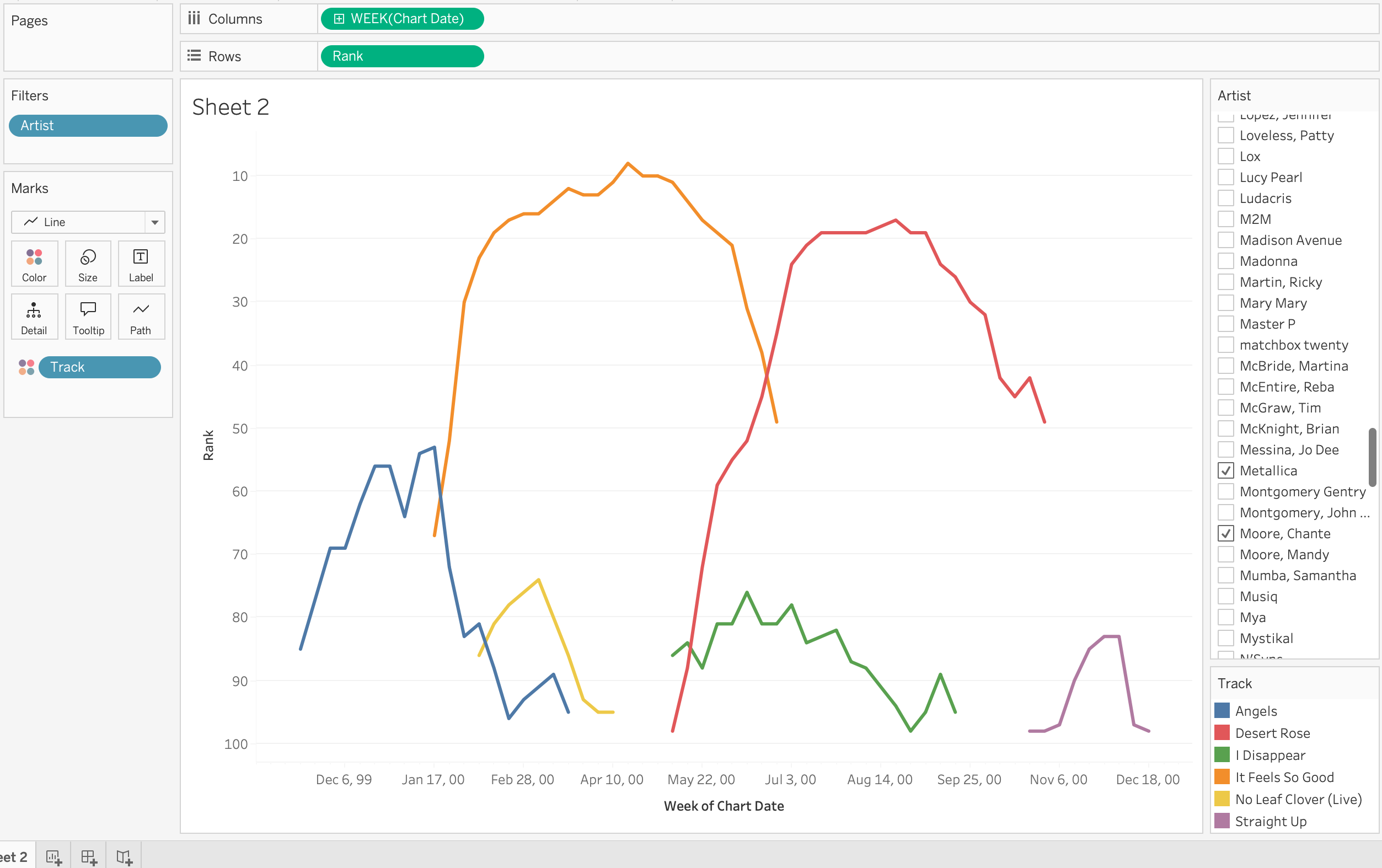
Worksheet 2: Song Trajectories (line chart)
Data source: billboard-long.csv
- Drag
chart_dateto Columns — Tableau may default to YEAR; right-click the pill and select WEEK(chart_date) to get weekly granularity - Drag
rankto Rows - Reverse the Y-axis: right-click the rank axis > Edit Axis > check Reversed (rank 1 at the top)
- Drag
artistto Filters > select 2-3 artists who had multiple songs (e.g., Metallica, Madonna). Show the filter as a dropdown: right-click the filter pill > Show Filter - Drag
trackto Detail on the Marks card (this separates lines per song) - Drag
artistto Color on the Marks card - Change Mark type to Line
- Title: “Song Trajectories”
Worksheet 3: Weeks on Chart (histogram)
Data source: billboard-songs.csv
- Right-click
weeks_on_chart> Create > Bins… > bin size 1 - Drag
weeks_on_chart (bin)to Columns - Drag
Number of Records(orCNT(track)) to Rows - Title: “Distribution of Weeks on Chart”
Part 3: Choose Your Own Worksheet
Pick at least one from the menu below.
| Chart | Difficulty | Data Source | Hints |
|---|---|---|---|
| Top 15 longest-running songs (horizontal bar) | Easy | songs | Color by peak_rank |
| New entries by month (bar) | Easy | songs | Derive month from date_entered |
| Peak rank vs. weeks on chart (scatter) | Medium | songs | weeks_on_chart on Columns, peak_rank on Rows. Add genre to Color |
| Rank x week heatmap | Medium | long | week on Columns, track on Rows, rank to Color. Mark type: Square. Filter to top 10 songs |
| Weeks on chart by genre (box plot) | Medium | songs | Use Show Me panel > box plot |
Part 4: Polish & Submit
- Titles: Every worksheet has a descriptive title
- Tooltips: Hover over marks — customize via Tooltip on the Marks card
- Sheet names: Rename tabs (not “Sheet 1”, “Sheet 2”)
- Save: File > Export Packaged Workbook (
.twbx) or save to Tableau Public
Your workbook should have at least 4 worksheets.
If time allows: explore freely
You have two datasets and a working Tableau setup. Think of a question about Billboard 2000 that interests you and try to answer it with a chart. Some starting points:
- Do longer songs tend to rank higher or lower?
- Which artists had multiple songs on the chart at the same time?
- Is there a relationship between when a song entered the chart and how long it lasted?
Build a new worksheet, pick the right data source, and see what you find. There are no wrong answers here — the goal is to practice turning a question into a visualization.