Calculating at the Right Level

BUS220 - Business Intelligence and Analytics | Week 5

Oleh Omelchenko

2026-04-06

Assumptions vs. evidence

“Last week you investigated a bikeshare dataset and found that what looked like a crisis — rides down 32% — was actually normal seasonality. The VP’s assumption was wrong, and the data showed it. That’s one kind of data mishap. Today we’ll see several more — and they all come down to the same thing: substituting assumptions for evidence.”

Two observations, one story?

Time A	Time B	What it looks like
22°C at 9am	22°C at 9pm	Stable temperature
1,200 rides in Oct	820 rides in Nov	Ridership crisis
62% life expectancy in 1960	75% in 2015	Steady improvement

Each row hides something. Let’s look at what’s between the endpoints.

“Each of these looks like a clean story told by two data points. The temperature is stable. Ridership is dropping. Life expectancy improved. But two points can hide anything that happened in between — and often they do.”

Endpoint illusions

Your apartment. 22°C at 9am. 22°C at 9pm. Perfectly stable, right?

Someone left the oven on for four hours. Two data points hid the entire event.

“The assumption: if the start and end are the same, nothing happened in between. Sounds reasonable — and it’s completely wrong here.”

“This is the same principle behind slopegraphs that connect 1960 to 2015 and declare ‘life expectancy improved everywhere’ — while hiding genocides and wars in between. You may have seen that example in the optional ADP reading. Two endpoints can mask anything.”

“The fix isn’t complicated: show the full timeline. But you have to know to ask for it — and that means not trusting the assumption that two points are enough.”

When the overall trend lies

Two exercise programs tested on 200 people. Overall results:

Program	People	Lost weight	Success rate
Yoga	100	62	62%
CrossFit	100	55	55%

Yoga wins. Recommend it to everyone?

“Clear result, right? Yoga has a higher success rate. If someone asked you which program to recommend, you’d say Yoga.”

Pause. “But what if we check who signed up for each program?”

Break it down by starting fitness

Starting fitness	Program	People	Lost weight	Success rate
Already active	Yoga	80	56	70%
	CrossFit	20	16	80%
Sedentary	Yoga	20	6	30%
	CrossFit	80	39	49%

CrossFit wins in both groups. Yoga looked better overall only because it attracted the easier-to-help population.

This is Simpson’s paradox — the aggregate reverses when you control for a hidden variable.

“CrossFit has a higher success rate among active people AND among sedentary people. But it loses overall because 80% of its participants were sedentary — the harder group. Yoga got the easier crowd.”

“The assumption: the overall winner must be better. The evidence: when you control for who was in each program, the story flips.”

“This happens in real data all the time — in hiring, in school test scores, in medical trials. The Berkeley admissions case is the most famous: UC Berkeley was sued for gender discrimination because men had a higher overall admission rate. But within every department, women were admitted at equal or higher rates. Women just applied to the more competitive departments.”

Simpson’s paradox, visually

The best way to build intuition for this is to see it move. Open this interactive and drag the grouping variable:

setosa.io/simpsons

Watch the overall trend reverse when you separate the groups — nothing changes except the level of analysis.

Detecting this requires looking at the data at two different levels — the aggregate and the segment. You need tools that let you control the grain of your calculation.

Open the setosa.io link on the projector. Let students watch or follow along on their phones/laptops for 1-2 minutes. The interactive makes the paradox visceral — you see the same scatter plot split into groups, and the regression lines flip direction.

“This is why the level of your analysis matters so much. And sometimes the right answer is ‘we don’t have enough data to check.’ If the exercise study hadn’t recorded starting fitness level, you couldn’t detect the paradox. Saying ‘I can’t answer this with what I have’ is not a failure — it’s the most honest analytical conclusion you can make.”

“So — we need tools that let us control the level of our calculations. That’s the rest of today’s lecture.”

The common thread

Mishap	The assumption	The check
Seasonal panic	“Month-to-month drop = crisis”	Compare year-over-year
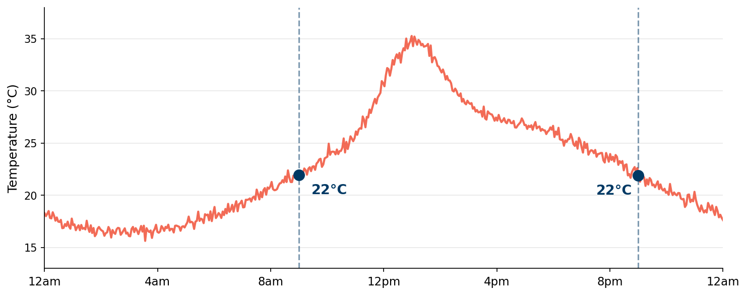
Endpoint illusion	“Start and end match = stable”	Show the full timeline
Simpson’s paradox	“Overall winner = winner everywhere”	Break down by subgroup

Each assumption sounds reasonable. Each one is wrong. The only way to tell is to check at a different level.

And sometimes the honest answer is: “We don’t have the data to check.”

“Three mishaps, one pattern: a reasonable assumption replaces a check you could actually run. In every case, the data was available to get the right answer — the analyst just didn’t look at the right level.”

“The ‘we don’t have enough data’ point is worth repeating. If you can’t segment, you can’t detect Simpson’s paradox. If you don’t have last year’s numbers, you can’t check for seasonality. Acknowledging that is not a failure — it’s what separates careful analysis from speculation.”

Not all calculations are equal

“Running totals, percent change, moving averages — none of these can be done with SUM or AVG. But they’re also not all the same kind of calculation. Let’s map out what’s actually going on.”

Four types of calculations

Layer	What it computes	Example	Depends on view?
Row-level	One value per row, before grouping	DATEDIFF(‘day’, [Order Date], [Ship Date])	No
Aggregate	Groups rows by dimensions in the view	SUM([Sales]), AVG([Profit])	Yes — changes with dimensions
Table calculation	Runs on the aggregated results	Running total, % of total, rank, MoM %	Yes — changes with layout
LOD expression	You specify the grain	{FIXED [Customer ID] : MIN([Order Date])}	No — ignores the view

“You’ve been writing the first two since week 4. Row-level: each row gets its own value, like adding a column in a spreadsheet. Aggregate: SUM, AVG, COUNT — computed after Tableau groups by whatever dimensions are on the shelves.”

“Today’s two new layers: table calculations run after aggregation, on the table of results you see on screen. LOD expressions let you specify the grain yourself — ‘compute this at the customer level, regardless of what’s in the view.’”

“The key difference between Layer 3 and Layer 4: table calculations depend on the layout — if you rearrange the view, the result changes. LOD expressions are stable — they always compute at the grain you specified.”

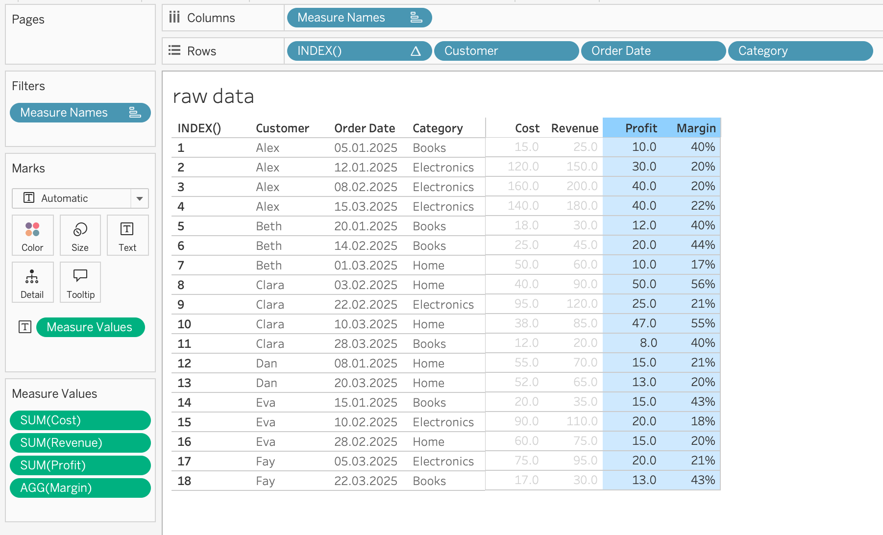
Layer 1: row-level — each row gets its own value

The Profit and Margin columns are row-level calculations: [Revenue] - [Cost] and ([Revenue] - [Cost]) / [Revenue]. Each row computed independently.

“18 orders, 6 customers, 3 categories, 3 months. Small enough to see everything at once. Let’s walk through all four layers on this data.”

“The profit and margin columns are row-level — each row gets its own result. Already you can see something: Books consistently has 40%+ margins. Electronics is 18-22%. The biggest revenue category is the least profitable per dollar. You’d never see this from an aggregate — you need the row-level detail.”

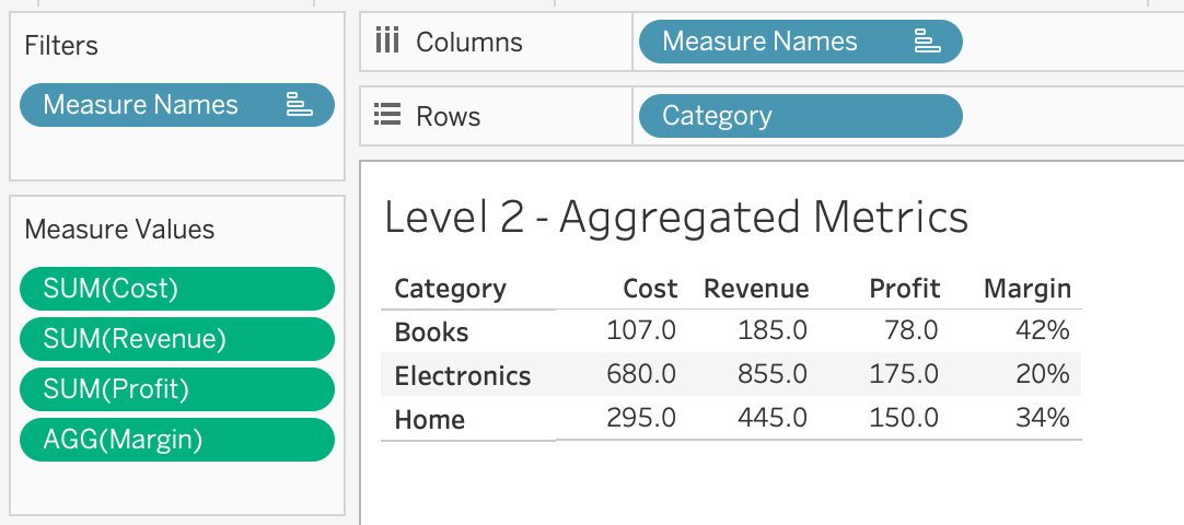
Layer 2: aggregate — what changes with the grouping

Group by category

Electronics leads revenue. Books leads margin.

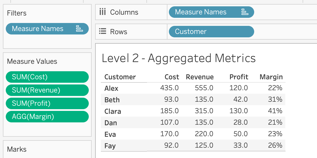
Group by customer

Alex is 37% of total revenue.

One formula — SUM([Revenue]) — but the grouping determines what you see.

“Same SUM formula, two completely different stories. The category view tells you Electronics dominates. The customer view reveals that one person — Alex — is 37% of your business. If Alex leaves, revenue drops by a third.”

“This is why aggregate calculations depend on the view. You already knew this from week 4. But watch what happens when we need something aggregation can’t do.”

Layer 3: table calculations — derived from the layout

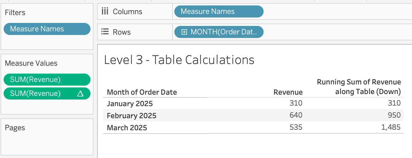
Running total — monthly revenue accumulates across months:

March dipped from February, but the cumulative trajectory shows the business is growing overall. This is how you answer the CFO who asks “are we going to beat last year?” — overlay two running totals and see where they cross.

“The running total tells a different story than the month-by-month view. March looks like a dip, but cumulatively we’re on track.”

“This is the calculation behind the BBoD Ch 10 dashboard — YTD and YoY on the same chart. Your CFO asks ‘are we on pace?’ and the answer is a running total comparison. You can’t build that with a regular SUM — you need a calculation that accumulates across the already-computed monthly totals.”

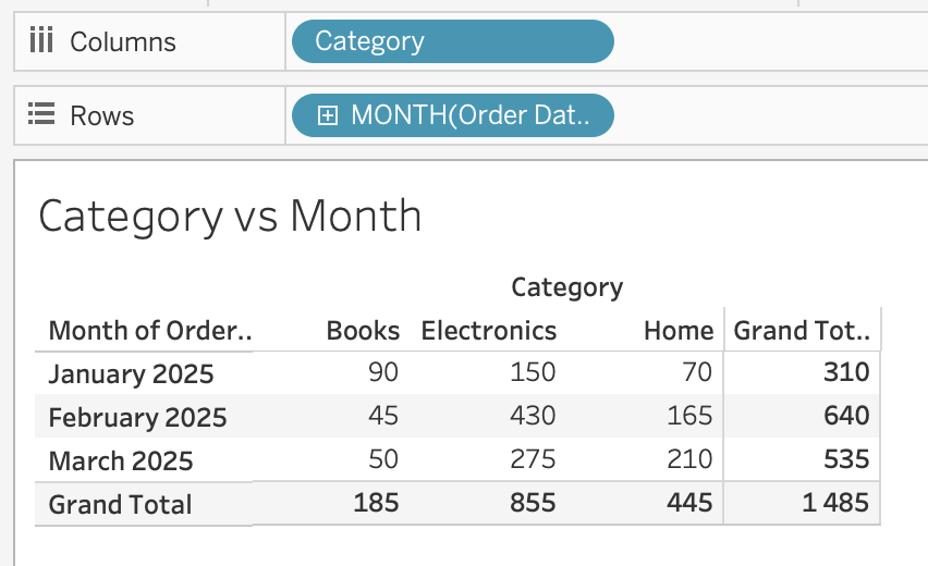
Layer 3: where is the mix shifting?

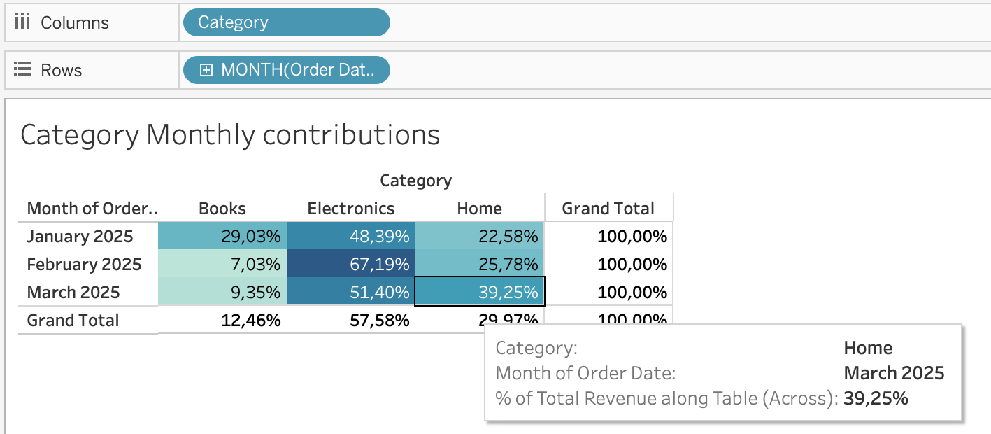
The same data, broken down by category per month — first as raw revenue, then as percent of total:

Books collapsed from 29% to single digits. Home grew from 23% to 39%. You wouldn’t see these shifts in the raw revenue totals on the left.

“The left table shows raw revenue — hard to spot the trend. The right table shows each row as a percentage across categories. Now the shift jumps out: Books collapsed, Home is growing.”

“This is a table calculation — percent of total, computed across the row. If you removed the Month dimension, the calculation would change completely. That’s what ‘view-dependent’ means.”

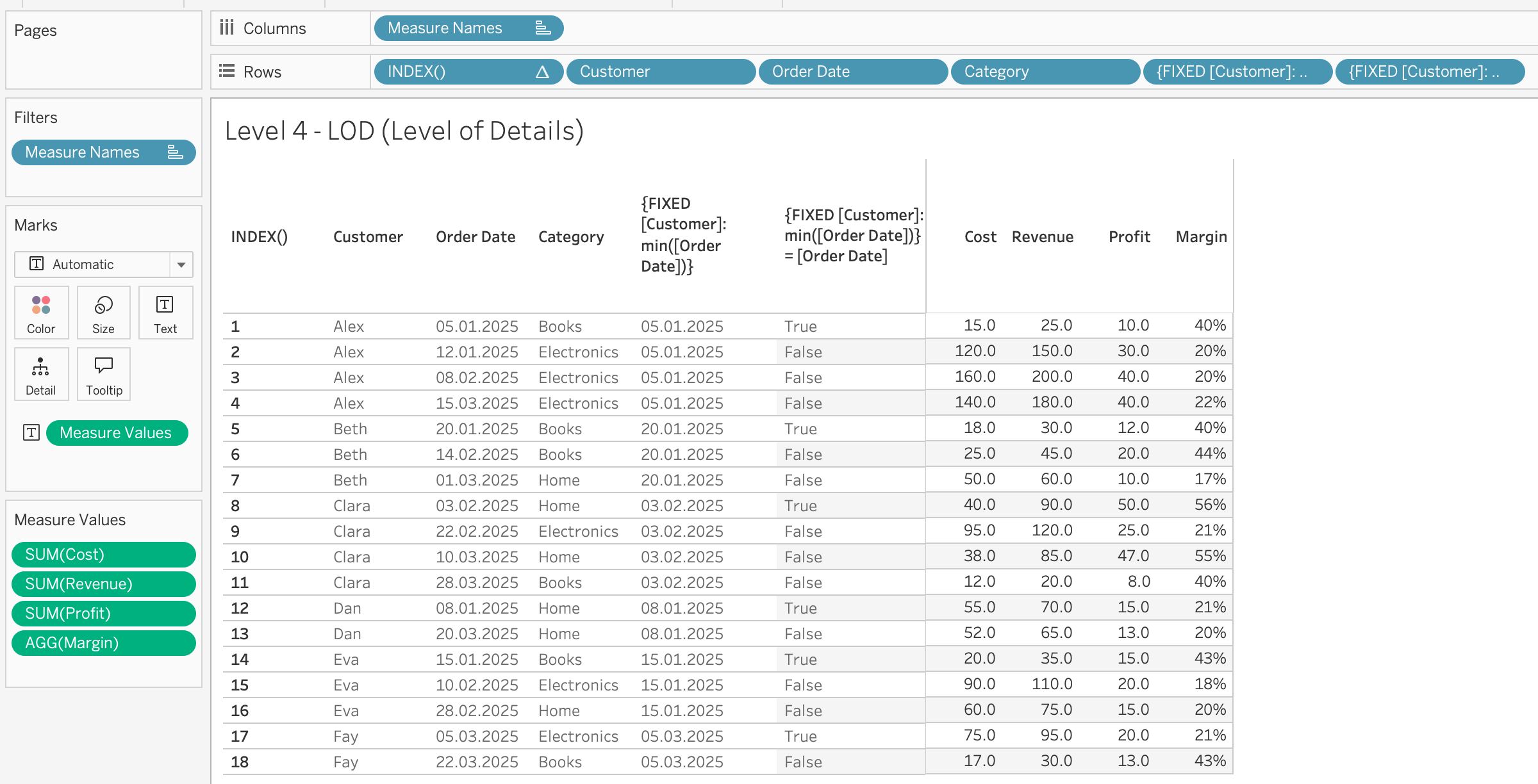
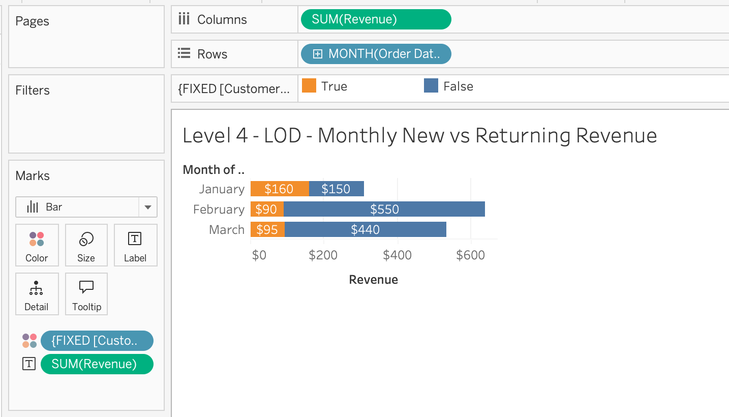
Layer 4: LOD — what the view can’t see

{FIXED [Customer] : MIN([Order Date])} — each customer’s first purchase date, attached to every row.

“Look at the two new columns. The FIXED expression computed each customer’s first purchase date — Clara’s is Feb 3, Fay’s is Mar 5, everyone else is January. The boolean column checks whether this order is from the customer’s first month.”

“This result stays the same no matter what dimensions are in the view. If you filter out January, Alex’s first purchase date is still Jan 5 — because the LOD runs before dimension filters. A regular aggregate would recalculate and give you the wrong answer.”

LOD in action: new vs. returning revenue

January is all new customers. By March, most revenue comes from returning customers — with only Fay as a new arrival.

“Once you have the FIXED first-purchase date and the new/returning flag, you can split revenue by customer type. January is 100% new — everyone is buying for the first time. By March, returning customers dominate.”

“You’ll build exactly this view on the Olist data in practice — and discover something very different. On Olist, almost no one returns. This tiny store has good retention; Olist doesn’t.”

“Notice what made this possible: the LOD computed a fact about each customer — their first purchase date — that doesn’t depend on the view. Without it, you couldn’t distinguish new from returning.”

The execution order

Data Source

→

LOD FIXED

→

Dimension Filters

→

Aggregation

→

Table Calculations

→

Table Filter

LOD runs early — before most filters. Aggregation happens next. Table calculations run last — on the results you see on screen.

“Now the pipeline makes sense concretely. You just saw it: the FIXED calculation survived the filter because it runs before filters are applied. The running total changed when we removed the Month dimension because table calculations run on whatever the view currently shows.”

“We’ll keep this simple for now. The full nuance — context filters, INCLUDE vs. EXCLUDE — comes later.”

Which layer do you need?

Mentimeter quiz — 4 questions, each with four options: Row-level, Aggregate, Table calculation, LOD expression. Reveal the distribution after each, brief discussion, then next.

Questions (build in Mentimeter):

1. “How many days did this delivery take?” → Row-level (DATEDIFF on two dates in the same row)
2. “What’s the average salary by department?” → Aggregate (AVG grouped by department)
3. “Did this team move up or down in the standings since last season?” → Table calculation (rank comparison across periods)
4. “Is this student scoring above or below their own average?” → LOD ({FIXED [Student] : AVG([Grade])}), then row-level comparison

Quiz time

For each question: which type of calculation do you need?

Row-level

Aggregate

Table calculation

LOD expression

Open Mentimeter. Give students 30 seconds to join. Then go through the 4 questions one at a time — reveal the distribution, brief discussion, next.

One question to decide

“If I add another dimension to this chart, should this number change?”

Yes → table calculation. The result depends on the view layout.

No → LOD expression. The result is fixed at the grain you specify.

“When you’re not sure which type to use, ask yourself this question. Percent of total — should it recalculate when you add a dimension? Usually yes — that’s a table calculation. Customer’s first purchase date — should it change when you rearrange the chart? No — that’s an LOD.”

“In practice you’ll use both, often in the same dashboard.”

Practice: diagnosing the Olist stagnation

You’re continuing with your Olist workbook from last week.

Last week you found the stagnation. This week you diagnose it — from two angles:

Products: group the 73 categories into macro-categories, then use table calculations to find where the decline is concentrated.

Customers: use LOD expressions to identify each customer’s first purchase date, split new vs. returning, and build a cohort retention view.

“The unresolved question from last week drives both sessions. You’ll need the readings — PT Ch 13 for table calculation mechanics, PT Ch 16 for LOD syntax — before you start.”

Mention that the LLM usage for category grouping is expected and consistent with the course AI policy.

“Reading for next week: PT Ch 14 (Parameters), PT Ch 15 (Sets), SWD Ch 3–4 (Clutter, Focus Attention).”