How We See Data

BUS220 - Business Intelligence and Analytics | Week 2

Oleh Omelchenko

2026-03-18

What do you remember from last week?

What is a dashboard?

What makes data “dirty”?

What was the one question this course keeps asking?

Open with a quick recall exercise. Give students 30 seconds to think, then take 2–3 answers.

You’re looking for: “a tool someone checks repeatedly to support decisions,” dirty data examples (duplicates, inconsistent formats, missing values), and “can someone make a decision from this?”

Once you’ve collected a few answers: “Good. So we know what a dashboard is, and we know the data underneath has to be clean. This week we ask a harder question: why do some ways of showing data work better than others? And the answer has more to do with biology than with design taste.”

How the brain sees data

Let’s start with a question that sounds simple but has a surprising answer: why are charts easier to read than tables?

A table of numbers

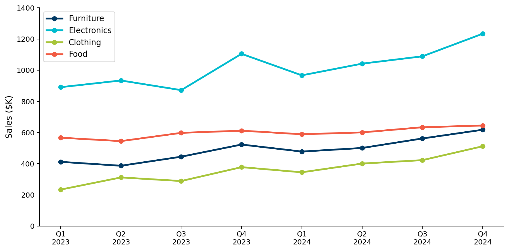
Look at these quarterly sales figures. Which category grew the most? Which quarter was worst?

Category	Q1 2023	Q2 2023	Q3 2023	Q4 2023	Q1 2024	Q2 2024	Q3 2024	Q4 2024
Furniture	412	387	445	523	478	501	562	618
Electronics	891	934	872	1,105	967	1,042	1,089	1,234
Clothing	234	312	289	378	345	401	423	512
Food	567	545	598	612	589	601	634	645

Take 10 seconds.

Put this up and give them 10 seconds. They’ll struggle — scanning 32 numbers and holding comparisons in working memory is hard.

After 10 seconds: “Tough, right? All the information is right there. But the format defeats the brain.”

The same data as a chart

Same 32 numbers, different encoding. Growth patterns and comparisons are now obvious.

Show the line chart. The answers are immediate: Clothing grew the most proportionally, Electronics has the highest absolute values, Q3 2023 had dips across multiple categories.

“You all know charts are easier to read than tables. Some of you studied this formally in data visualization. Today I want to go one level deeper: why does the chart work? What’s happening in your brain?”

Three types of memory

How your brain processes what it sees:

Iconic (sensory) memory — a visual snapshot, lasts a fraction of a second. This fires when you first look at a chart.

Short-term memory — lasts seconds, holds roughly 4–7 items. This is why you couldn’t process 32 numbers — it overflowed.

Long-term memory — effectively unlimited, but slow to encode. Stores familiar patterns like “up and to the right means growth.”

This is from Communicating with Data, Chapter 1. Three types of memory, each with different capacity and speed.

Iconic memory is the visual snapshot — it captures the whole scene in a fraction of a second. Short-term memory can hold about 4 to 7 items. Long-term memory stores patterns you’ve seen before.

The main point: a chart works when it compresses many data points into a pattern that fits in short-term memory. Four colored lines are four items — your short-term memory can handle that. But 32 individual numbers? Way over capacity.

This might be new for everyone — even if you’ve taken data viz, the cognitive science behind it usually isn’t covered in detail.

Why the chart worked

The line chart compressed 32 numbers into 4 visual patterns (lines) that fit in short-term memory.

A well-designed chart chunks data for you. It groups items into patterns you can hold in memory.

A bad chart fails when it forces the viewer to hold too many unrelated items at once.

Chunking is the key concept here. A line chart groups 8 data points into one visual object — a line with a shape and direction. Four lines, four chunks, well within short-term memory capacity.

A bad chart — say, 32 separate bars with no grouping — doesn’t chunk for you. It presents 32 items and hopes you can hold them all. You can’t.

Pre-attentive attributes

What the eye processes before you think.

Now we get to the mechanism that makes charts work at the most basic level — pre-attentive processing. If you took data viz, you’ll recognize the term. What we’ll focus on here is the mechanism — why it works, and what it means for choosing how to display data.

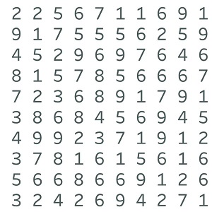
Count the 9s

How many 9s? Count them. Take 10 seconds.

Put up the grid and ask students to count the 9s. Give them 10 seconds.

They’ll take time and likely get it wrong. This requires serial scanning — item by item, engaging short-term memory for each digit. It’s slow and error-prone.

“Having trouble? That’s normal. You’re scanning one digit at a time because nothing makes the 9s stand out from the rest.”

This demo is from Big Book of Dashboards, Chapter 1, Figures 1.6–1.8.

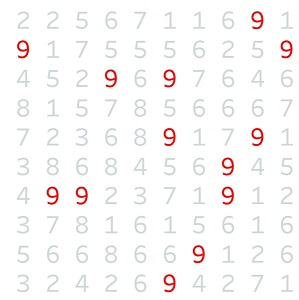
Now count the 9s

The answer is instant — your brain detected them before you consciously read any digit.

Same grid, but the 9s are colored red. The answer is instant — the 9s “pop out” without effort.

This is pre-attentive processing. The color difference is detected in under 250 milliseconds — before conscious attention kicks in. Your visual system flagged “different!” before your conscious mind even started reading digits.

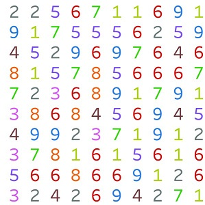
Too many colors

The pop-out effect disappears when everything competes for attention.

Now every digit has a random color. Try finding the 9s. Much harder — the pop-out effect is gone because too many colors compete for attention.

The lesson: pre-attentive attributes work when used selectively. One highlight color works. Ten colors create noise. This is one of the most common mistakes in dashboard design — using too many colors because it looks “more informative.”

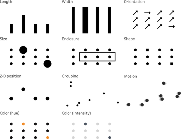
Pre-attentive attributes

The brain detects these features in under 250 milliseconds:

This is worth a photo — you’ll reference it all course. (CwD Ch1 Figure 1-3)

This is the catalog of pre-attentive attributes from Communicating with Data, Chapter 1. Tell students it’s worth taking a photo.

“I’ll move through this quickly — those of you who took data viz have seen this catalog. For everyone else, the readings cover each attribute in detail. What matters for today is the hierarchy — not all attributes are equal.”

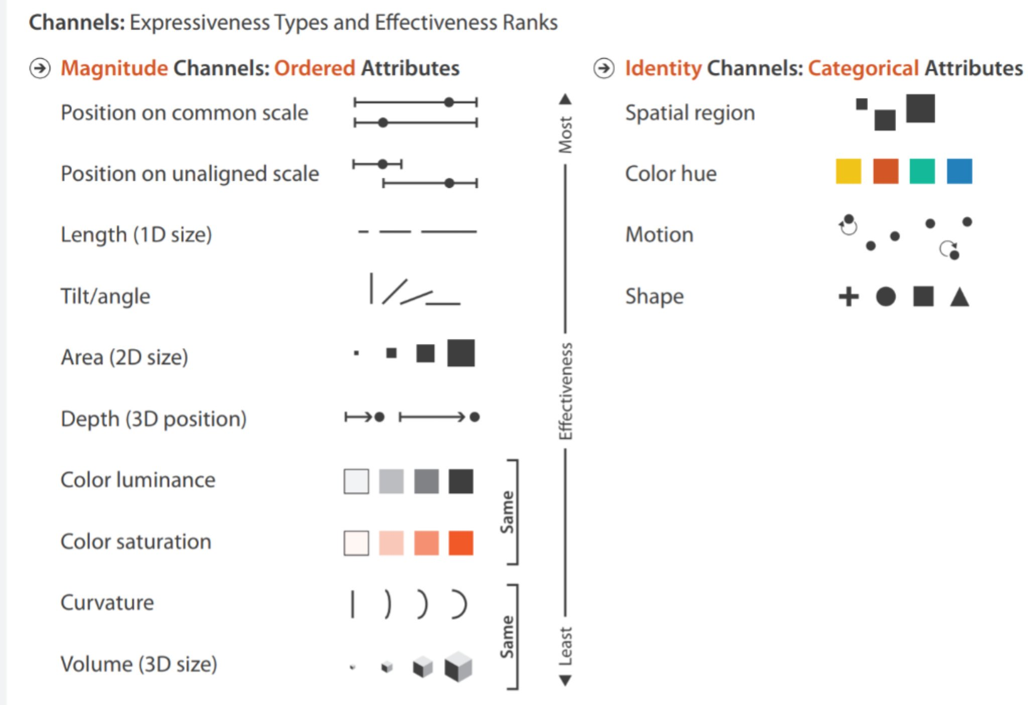
Not all attributes are equal

Magnitude channels (left) are ranked by precision. Position and length are at the top — you can tell one bar is exactly 20% longer than another. Color and size are at the bottom — you can see “darker” or “bigger” but can’t quantify how much.

Identity channels (right) encode categories. Spatial region, color hue, and shape tell you “this is different from that.”

This ranking explains most chart design rules.

This ranking comes from Visualization Analysis and Design (Munzner) and aligns with the Stephen Few hierarchy in CwD Chapter 1. The left column shows ordered/magnitude attributes ranked from most to least precise. The right column shows categorical/identity attributes.

Bar charts beat pie charts because length (high on the list) beats angle/area (low). Scatterplots are powerful because position on a common scale is the single most precise channel. Color hue is good for categories, but you can’t use it to encode quantities precisely.

If you took data viz, you learned these as rules. Now you know the perceptual science that generates them. For everyone else, BBoD Chapter 1 and CwD Chapter 1 cover this in detail.

Data is not reality

So the visual system is powerful — it finds patterns fast. But there’s a trap: if the data is wrong, the visual system will find patterns in the wrongness, and you’ll believe them.

Last week we talked about dirty data — duplicates, formatting errors, missing values. That’s the mechanical side. Today I want to talk about something more fundamental.

Two quotes

“All models are wrong, but some are useful.”

— George Box, statistician

“Plans are useless, but planning is indispensable.”

— Dwight Eisenhower

What do these have in common? And what does either of them have to do with data?

Put both quotes up and give the room 30–60 seconds. Take 2–3 answers.

What they have in common: both say that the representation (a model, a plan) will always be incomplete or wrong — but the process of building it is still worth doing. A model simplifies reality on purpose. A plan will change on contact with reality. Both are useful despite being imperfect.

The connection to data: every dataset is a model of reality. It’s a simplified, incomplete representation — and it’s wrong in ways you might not notice. But it’s still useful, as long as you understand how it’s wrong.

This is the mindset shift for this block: we move from “is the data clean?” (last week) to “even if the data is clean, how faithfully does it represent what actually happened?”

If students struggle, prompt: “What does a model leave out? What does a plan assume?” Then connect to: “What does a dataset leave out? What does it assume?”

Data and reality are not the same thing

Every dataset is a model — a simplified, incomplete representation.

It records what was observed, reported, and stored, not what actually happened.

That gap is always there. The question is how big it is and whether you’ve thought about it.

This is the core idea of Avoiding Data Pitfalls, Chapter 2. Every dataset is a proxy for reality, not reality itself. The data tells you what was recorded by a particular process at a particular time, and that process has its own biases and blind spots.

Connect back to Box: the dataset is “wrong” — it’s an imperfect representation. But it can still be “useful” if you understand the limitations.

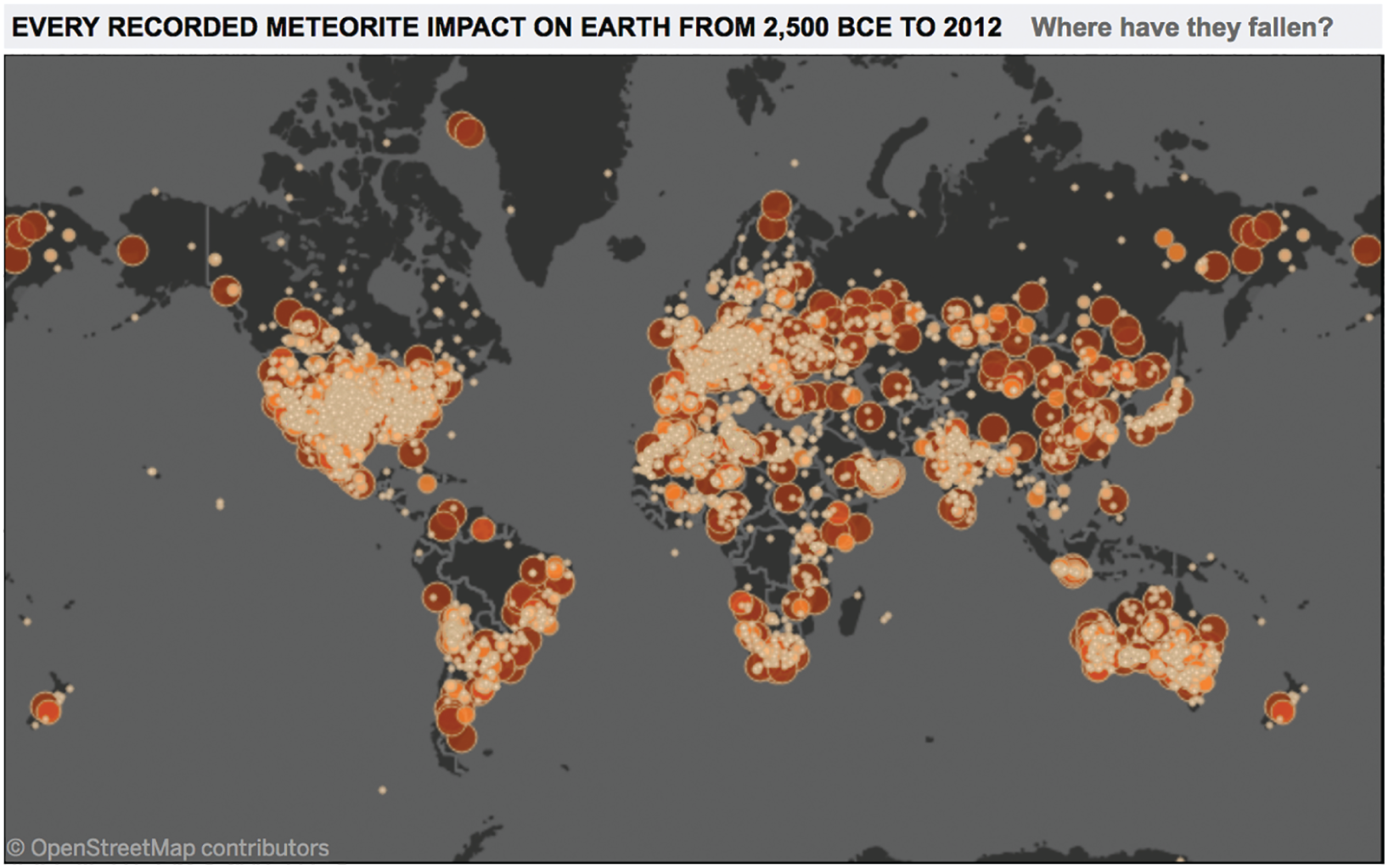
Where meteorites fall

What pattern do you see?

This is from Avoiding Data Pitfalls, Chapter 2 (pp. 30–34). The Meteoritical Society database: 34,513 recorded meteorite impacts from 2500 BCE to 2012.

Show the map and ask: what pattern do you see?

Students will notice clusters in North America, Western Europe, parts of Australia and Japan — and near-empty zones in oceans, Central Africa, Central Asia, and the Amazon.

“Do meteorites avoid the ocean? Do they prefer Western Europe?”

A map of observation

The clusters match population density and scientific institutions.

This map shows where someone was standing nearby, noticed a meteorite, and reported it to a database.

The data is real. But a perfectly accurate visualization of the data tells a story about record-keeping — about where scientific institutions exist and where people live.

Of course meteorites don’t prefer Western Europe. This map shows where someone was standing nearby, noticed a meteorite, and reported it to a scientific database. It’s a map of observation infrastructure.

“Every dataset has a version of this problem. When you see ‘website traffic went up 40%,’ ask: did more people visit, or did we start counting differently? When you see ‘customer complaints dropped,’ ask: did complaints decrease, or did we make the complaint form harder to find?”

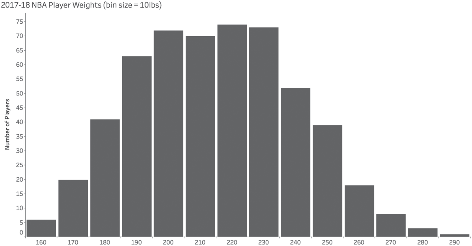
Human-entered data looks fine at a distance

NBA player weights at 10-pound bins. Looks smooth, looks normal. Nothing suspicious.

From ADP Chapter 2 (pp. 38–41). Show this histogram first — it looks perfectly fine. A normal, slightly right-skewed distribution of NBA player weights. Everything seems clean.

“Looks reasonable, right? Nothing suspicious. Now let’s zoom in.”

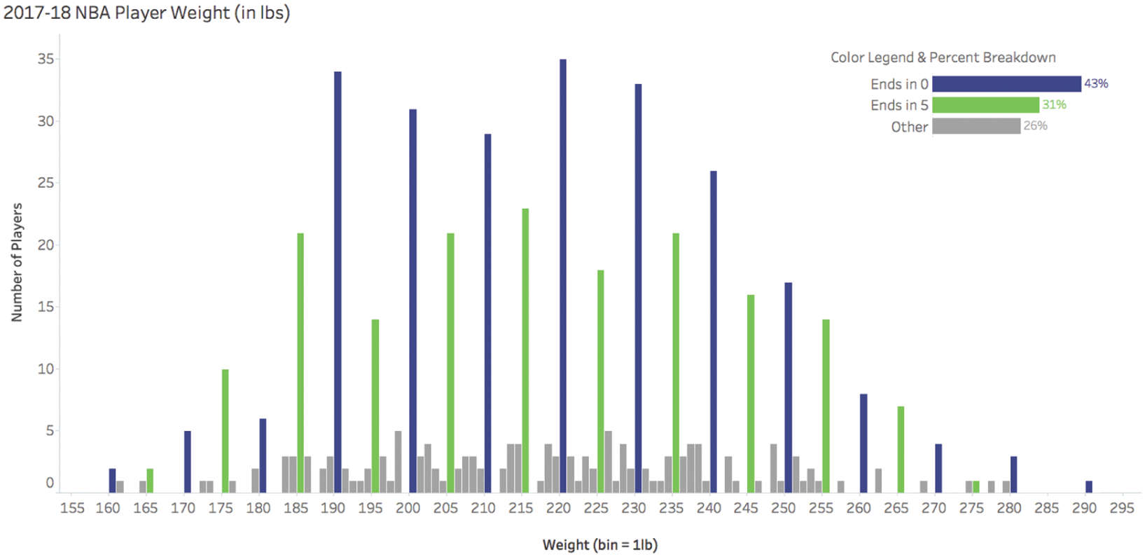
Zoom in and the rounding appears

At 1-pound bins: 43% of entries end in 0, and 31% end in 5. Only 26% fall on other digits.

Nobody weighs exactly 200.0 pounds. These are human-entered approximations.

Same data, 1-pound bins. Massive spikes at weights ending in 0 (blue, 43%) and 5 (green, 31%). Only 26% of entries end in other digits.

Someone eyeballed the scale, rounded to the nearest 5 or 10, and typed it in. Contrast this with NFL Combine data, where players are precisely measured by staff using calibrated equipment — the last-digit distribution is nearly uniform. Same type of data, completely different reliability. The difference is the process: self-reported vs. professionally measured.

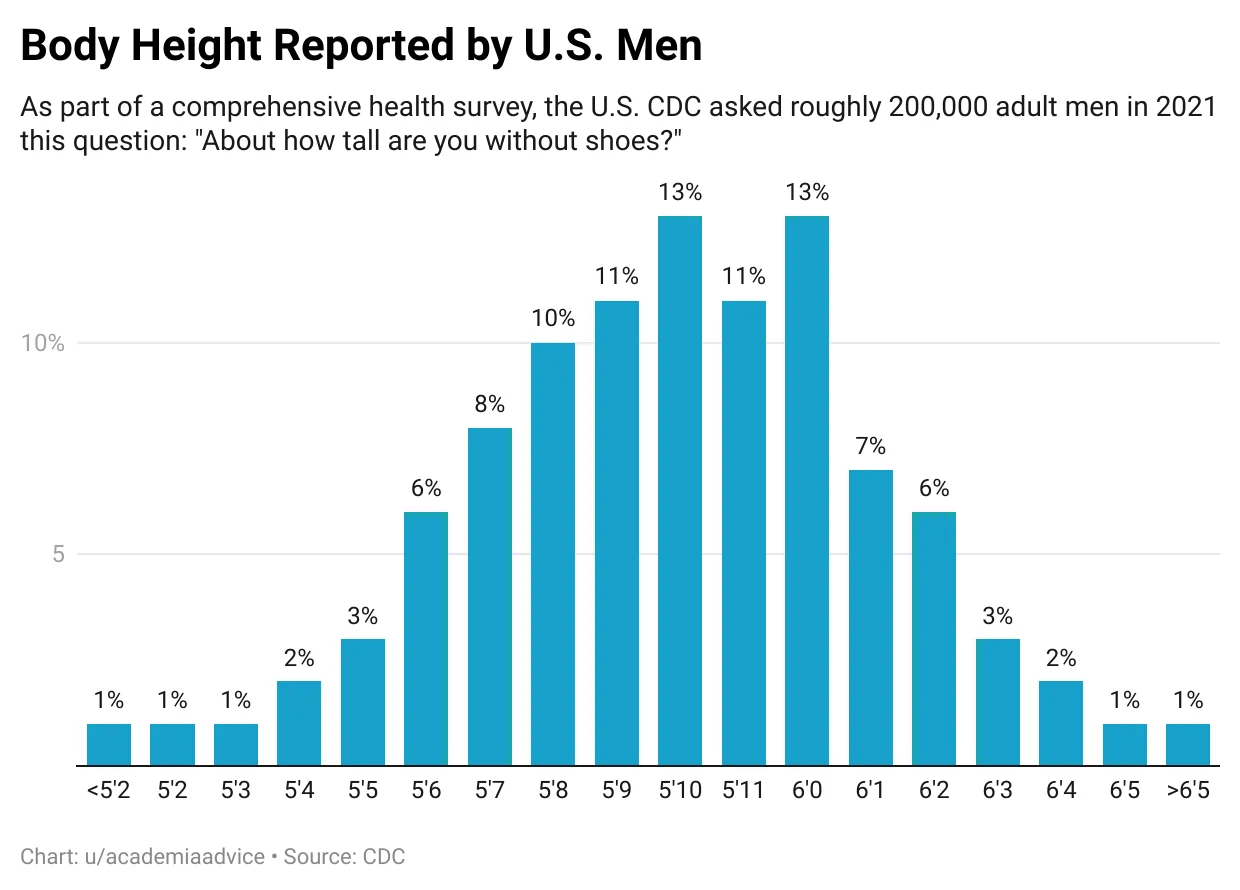
The same pattern in self-reported height

CDC survey, ~200,000 U.S. men, 2021. Spikes at 5’10”, 5’11”, 6’0” — people round up to the nearest “nice” number.

Same phenomenon as NBA weights, different domain. The CDC asked about 200,000 men “how tall are you without shoes?” — the distribution spikes at round heights, especially 5’10”, 6’0”, and 6’1”.

People don’t measure themselves precisely. They remember a number from years ago, or they round to what sounds right. The data is real — these are actual survey responses — but it reflects how people think about their height, not their actual height.

This is a quick reinforcement: the rounding bias pattern appears everywhere human-entered data exists. You’ll see it in ages, prices, timestamps, distances.

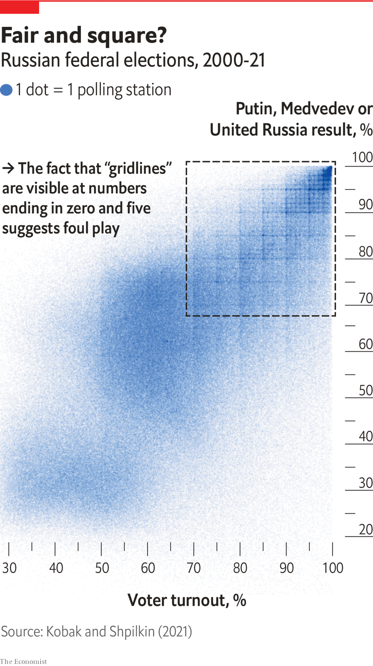
When rounding reveals something bigger

Russian federal elections, 2000–2021. Each dot is a polling station. The x-axis is voter turnout, the y-axis is the result for Putin, Medvedev, or United Russia.

Ask students: “What do you see?”

The visible “gridlines” at numbers ending in 0 and 5 — especially in the upper-right corner (high turnout, high vote share) — form a checkerboard pattern. This is the same rounding artifact we saw in NBA weights and body height, but it shouldn’t be there. Turnout and vote share are calculated from vote counts, not self-reported. If 347 out of 500 registered voters show up, turnout is 69.4%, not 70%.

The fact that results cluster at round numbers (70%, 75%, 80%, 85%, 90%, 95%, 100%) means someone wrote down the target number first and worked backward to the vote counts. This is statistical evidence of systematic fraud — from Kobak and Shpilkin (2021), published in a peer-reviewed journal and covered by The Economist.

The point for students: the same “what process generated this data?” question applies everywhere. In NBA data, rounding is harmless — someone was lazy with a scale. In election data, rounding is evidence of fabrication. The analytical skill is the same: look at the data generation process.

This is also a good moment to note: Ukraine’s election data, when analyzed the same way, does not show this pattern. Clean elections produce smooth scatter plots.

One rule before any analysis

Ask: what process generated this data?

Who collected it? How? Why?

The answer shapes what you can and can’t conclude.

You built a Profit Margin column last week by dividing Profit by Sales. That assumes both numbers are correctly recorded. In the Superstore dataset they are — it’s clean sample data. In a real company, Sales might be recorded at the point of sale, but Profit might be calculated monthly with estimated costs.

One rule: before you analyze any dataset, ask what process generated this data. Who collected it, how, and why? The answer shapes what you can and can’t conclude.

Connect back to week 1 practice: the Profit Margin formula assumed both numerator and denominator were reliable. In sample data they are. In real business data, different numbers come from different systems with different update frequencies and different levels of precision.

Audience and purpose

Before you build anything.

So we know the brain can process visuals fast, and we know the data might not be what it claims. The next question: who are you showing this to, and why?

This part is new for everyone — regardless of what courses you’ve taken. Data viz courses teach you how to make a good chart. They rarely teach you how to figure out whether you should be making a chart at all.

Exploratory vs. explanatory

Exploratory analysis is what you do at your desk. You filter, pivot, make 20 charts, try different angles. Most of what you try leads nowhere.

Explanatory analysis is what you present. The 2–3 findings that matter, with context and a recommendation.

Storytelling with Data calls this “opening 100 oysters to find 2 pearls.” Your audience wants the pearls. They don’t want to watch you open oysters.

The most common mistake in junior analyst work: presenting the exploration instead of the conclusion.

From SWD Chapter 1. The oyster analogy.

When you’re analyzing data, you try many things — you open 100 oysters to find 2 pearls. The mistake is showing your audience all 100 oysters. They don’t want your process. They want the 2 or 3 findings that matter, presented clearly with context.

Every chart in a presentation should be there for a reason, and the reason should not be “I made it during my analysis.”

Three questions before you build

WHO

Who specifically will use this?

What do they already know?

What do they care about?

WHAT

What action should they take?

Approve a budget? Change a process? Investigate a problem?

HOW

How does data support the point?

Data is evidence for your recommendation.

From SWD Chapter 1. Before you build anything — a chart, a dashboard, a report — answer these three questions.

The second one is the hardest: what action do you need? If you can’t name the action, you’re not ready to build. SWD provides a list of action words: accept, agree, begin, change, continue, fund, invest, pursue, stop.

This framework will show up in every assignment’s documentation component. When you explain your analytical choices (the 30% documentation grade), this is what I’m looking for.

The Big Idea

Distill your message to one sentence with three properties:

1. It states your unique point of view
2. It conveys what’s at stake
3. It’s a complete sentence — not a topic, not a title

Type	Example
Topic	“Shipping performance.”
Title	“Q4 shipping delays.”
Big Idea	“Q4 shipping delays cost us $200K in refunds and we need to switch carriers before peak season.”

From SWD Chapter 1, drawing on Nancy Duarte’s Resonate. The Big Idea is one sentence that captures your point of view, the stakes, and the action.

The difference between a topic and a Big Idea is the difference between “here’s some data” and “here’s what we should do about it.” Topics are passive. Big Ideas drive action.

Write a Big Idea

Situation: Your manager asks you to look into customer returns.

Your finding: 60% of returns come from one product category.

Write one sentence that includes:

• your point of view (what you think is going on)
• what’s at stake (why it matters)
• a recommended action (what to do about it)

Give them 2 minutes. Instruct them to work with neighbors. Walk around, listen. Then ask 2-3 pairs to share.

Good answers will look like: “Our electronics category drives 60% of all returns, costing us $X per month — we should audit product descriptions and return reasons before the holiday season.”

Weak answers will be topics: “Customer returns are a problem” or titles: “Returns by category.” Push them toward the action — what should someone do with this information?

Five Whys: dig past the surface request

Sometimes what the stakeholder asks for isn’t what they actually need.

“I need to know how many students we have.”

Why? “To plan room assignments.”

Why? “Building C renovation — we’re losing three classrooms.”

Why does that affect assignments? “Some classes might not fit.”

What do you actually need? “Which classes won’t fit in the remaining rooms after renovation.”

The original request would have produced a single number. The real need requires enrollment by class, room capacity, and a comparison.

From CwD Chapter 2. The Five Whys technique — originally from Toyota’s manufacturing process — helps you dig past the surface request.

The original request was “how many students do we have?” — that produces one number. But the real need is a comparison between class sizes and remaining room capacities. Completely different analysis, completely different deliverable.

You won’t always need all five “whys.” Sometimes one is enough. The point is to ask at least once before you start building. This connects directly to the documentation component of assignments — showing that you understood the real question, not just the surface request.

Choosing the right visual

Now you know how the brain works, you’ve questioned the data, and you know your audience. Time to pick the right visual.

Some of you covered chart selection in data visualization. I won’t repeat that material. Instead, I want to focus on three things: when you don’t need a chart at all, why certain chart types fail perceptually, and color as a design system. If you haven’t taken data viz, SWD Chapter 2 and BBoD Chapter 1 are your essential reading this week.

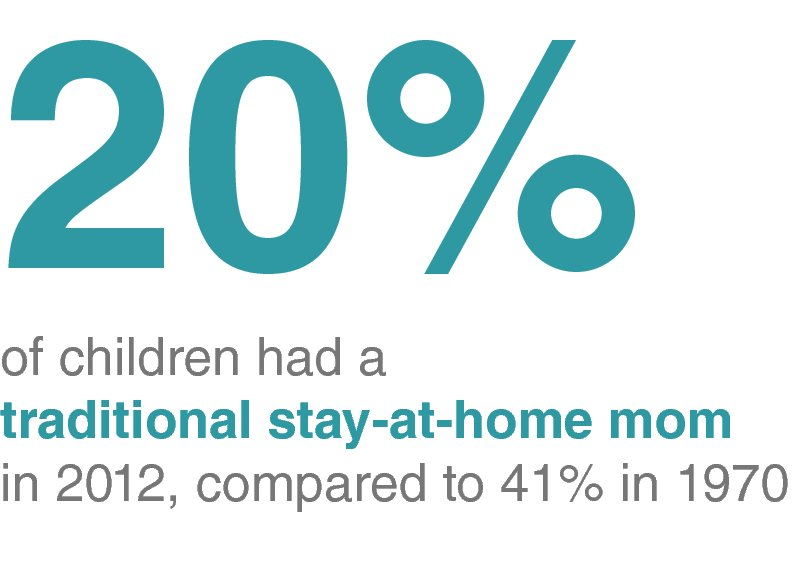
Sometimes you don’t need a chart

If you have one or two numbers, just make the number big.

The KPI tiles at the top of every business dashboard follow this pattern: one big number, a comparison, and a label.

From SWD Chapter 2 (pp. 2–3). The Pew Research example on the left is a bar chart showing two values — 41% in 1970 and 20% in 2012. It’s not wrong, but it’s a lot of visual machinery for two numbers.

The makeover on the right communicates the same data more directly: one big number with context. Your eye goes straight to “20%” and the comparison to 41% is right there in the text.

This is a scorecards principle, central to dashboard design. If a single number answers the question, respect that simplicity.

Tables vs. charts

Table — verbal system, cell by cell. Slow, precise. Use when exact numbers matter.

Chart — visual system, patterns at a glance. Fast, approximate. Use for trends and comparisons.

Heatmap — both: exact numbers + color patterns. Adding a color scale in a spreadsheet builds a heatmap.

From SWD Chapter 2 and BBoD Chapter 1. Tables and charts serve different purposes, and neither is better. Tables interact with the verbal system, charts with the visual system.

A heatmap gives you both — it’s a table with pre-attentive color intensity applied. This is why heatmaps are so effective for dense data: you get the exact numbers when you need them and the patterns when you don’t.

Design principle for tables: let the data stand out, not the borders. Light or minimal borders, clean alignment. Every pixel of ink that isn’t data is competing for attention.

Bar and line charts

Bar charts encode value as length — the most precise attribute.

• Horizontal for categories, vertical for time
• Always start at zero — truncated bars lie

Line charts encode value as position, change as slope.

• Use for continuous data (almost always time)
• Slope = rate of change
• Don’t connect categories with lines

Bar charts are everywhere for a reason: length is the most precisely assessed pre-attentive attribute. Two rules: horizontal for categories because labels read naturally, vertical for time because time flows left to right. And always start at zero — this is non-negotiable.

Line charts use position and slope, the second most precise attribute. Slope tells you rate of change — steeper means faster growth. But only use them for continuous data, almost always time. Connecting categorical points with a line implies continuity between the categories, which is misleading.

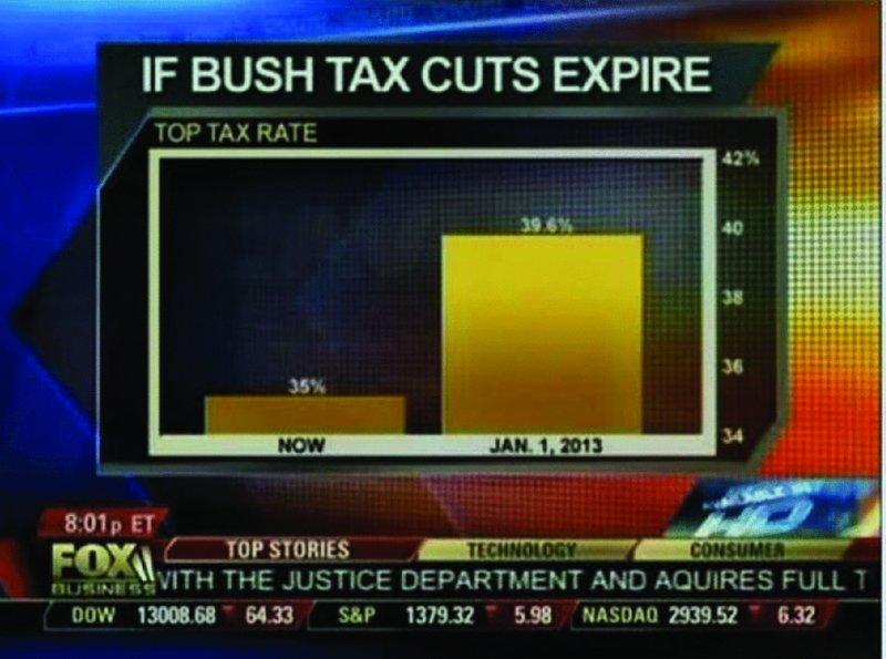
Zero baseline rule

This aired on Fox News. What’s wrong with it?

Show the TV screenshot first and let students spot the problem. The y-axis starts at 34%, making a small change from 35% to 39.6% look like an enormous jump.

“What’s wrong with this chart? Take a few seconds.”

Students will likely spot the truncated y-axis. This is probably the most famous misleading chart in data viz — from SWD Chapter 2, Figure 2.5.

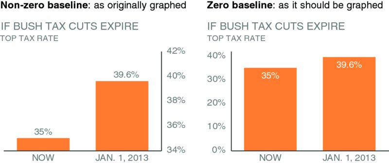
Non-zero vs. zero baseline

Left: y-axis starts at 34% — the change looks like a 460% increase.

Right: y-axis starts at 0 — the change is actually 13%.

The deception works because our brains read bar length automatically.

The corrected version on the right starts at zero. The same data now looks like what it is — a modest increase from 35% to 39.6%.

If you’ve seen this before, notice how it connects to Part 1: the deception works because our brains read bar length pre-attentively. We can’t turn off that processing. A truncated axis exploits that automatic response.

The fix is simple: start at zero. If the differences look too small at zero, that’s informative — maybe the differences really are small.

What fails and why

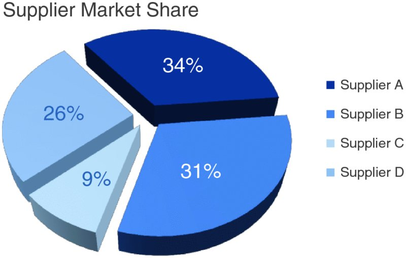
Pie charts — angle and area are imprecise. You can spot 25% and 50%, but 31% vs. 34%?

3D charts — shadows and perspective distort values. Every pixel that isn’t data is noise.

Dual y-axes — two scales on one chart imply false correlations and confuse the reader.

Three chart types that people use despite perceptual evidence against them.

Pie charts ask you to compare angles and areas — attributes low on the effectiveness hierarchy. A bar chart with the same data uses length, far more precise. We’ll see a direct comparison on the next slides.

3D charts add ink that isn’t data. Every shadow, floor plane, and side panel competes for attention and distorts values. Never use 3D unless you’re actually plotting a third dimension.

Dual y-axes force extra cognitive work — which axis goes with which data? The visual overlap can imply a correlation that doesn’t exist. Better alternatives: label data points directly, or stack two charts vertically with a shared x-axis.

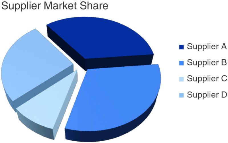
Pie chart: which supplier is bigger?

Can you tell which supplier has the largest share?

What about second largest?

How confident are you?

Show the 3D pie without labels first. Students will struggle to rank the suppliers — the 3D perspective makes it nearly impossible to compare the slices accurately. Supplier A and B are close, and the 3D distortion makes the front slices look larger.

“Look at this for a few seconds. Which supplier has the biggest share? Second biggest? How sure are you?”

Let them struggle for a moment before moving to the next slide.

Add labels — does it help?

Now you can read the numbers: 34%, 31%, 26%, 9%.

But if you need labels to understand the chart, the chart isn’t doing its job.

You’re reading a table arranged in a circle.

Same pie, now with percentage labels. The labels make the data accessible — but that’s the point. If the visualization only works because you added text labels, the visual encoding (angle, area) isn’t carrying the information. You’re reading numbers, not seeing patterns. The chart is just a table arranged in a circle with extra ink.

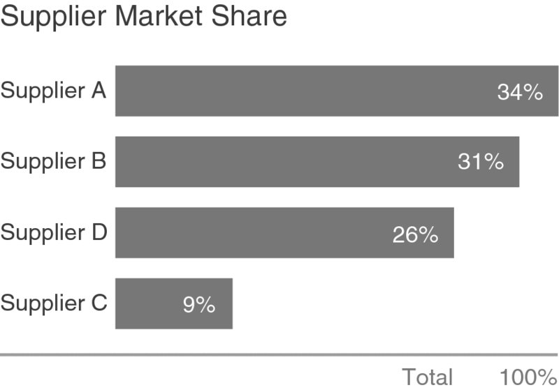
Same data as a bar chart

Same data. You can see the ranking without reading any labels.

Bar chart uses length (most precise attribute). Pie chart uses angle and area (least precise).

From SWD Chapter 2, Figures 2.13–2.15. The same supplier market share data as a horizontal bar chart.

The ranking is immediately obvious. You can see that A and B are close, D is about three-quarters of B, and C is small. No labels needed for the comparison — though they’re helpful for exact values.

This is the perceptual hierarchy in action: length beats angle beats area. The bar chart shows at a glance what the pie chart needed labels to convey.

Color as a design system

Type	Purpose	Example
Sequential	Light → dark for low → high	Heatmaps, choropleth maps
Diverging	Two colors from a midpoint	Profit/loss, above/below target
Categorical	Different hues for groups	Product lines, regions
Highlight	One color, rest gray	Drawing attention to one bar
Alert	Bright color for warnings	The check-engine-light from Week 1

From BBoD Chapter 1. Five uses of color, each serving a different purpose. Mixing them creates confusion.

Sequential scales are for ordered quantities — light to dark, low to high. This is what you use in heatmaps and conditional formatting.

Diverging scales have two colors meeting at a neutral midpoint — perfect for profit/loss or above/below target.

Categorical colors use different hues for different groups. The key rule: limit to 5-7 categories. More than that and the colors become indistinguishable.

Highlight color is underused: make one element stand out by graying out everything else.

Alert color is the check-engine-light principle from Week 1 — invisible until something needs attention.

In dashboards, you’ll often need all five on the same screen. The discipline is using each intentionally.

Color accessibility

About 8% of males and 0.4% of females have some form of color vision deficiency — mostly difficulty distinguishing red from green.

In this room, that’s statistically 1–2 people.

Practical rule: don’t encode meaning with red vs. green alone.

Use blue vs. orange instead, or add a second channel (shape, label, pattern) so the chart still works without color.

BBoD Chapter 1 recommends blue and orange as the safest two-color combination.

If you haven’t taken data viz, this might be the first time you’ve seen a CVD simulation. If you have — how many of you actually use blue-orange in practice? This is one of those rules that’s easy to know and hard to follow.

The practical rule: never use red vs. green as the only way to distinguish categories or encode meaning. Either use blue and orange, or add a second channel — labels, shapes, or patterns — so the information survives without color.

What’s ahead

Let me preview what’s coming in practice and what to read.

This week in practice

We’ll build a proto-dashboard in a spreadsheet — charts, conditional formatting, lookup formulas, structured layout.

It won’t be Tableau. But you’ll see how all the pieces connect: data in one sheet, analysis in another, a summary page someone else can read.

Every BI tool — Tableau, Power BI, Looker — does the same things under the hood. Spreadsheets make the mechanics visible.

The practice sessions this week use Google Sheets. Students will build conditional formatting (choosing pre-attentive attributes), use INDEX-MATCH for lookups, create charts, and structure an analytical report.

The point is to see the internal mechanics that BI software hides. When you drag a dimension onto Rows in Tableau, something similar to a pivot table happens. When you add a color scale in Tableau, it’s the same color intensity attribute we discussed today. Starting in spreadsheets makes these connections explicit.

Reading assignments

Everyone should read:

• SWD Ch1 — audience, Big Idea, storyboarding. The frameworks from today, in full detail.
• ADP Ch2 — the data-reality gap. More examples and a systematic framework.

If you haven’t taken data visualization:

• SWD Ch2 — chart types, what to avoid. The full chart-by-chart guide.
• BBoD Ch1 — pre-attentive attributes, color theory, encoding.

If you have taken data visualization:

• CwD Ch1 — the cognitive science behind pre-attentive processing.
• CwD Ch2 — data types, requirement gathering, the Five Whys.

Starting Week 3, quizzes will include reading material.

The readings are tiered. Everyone should read SWD Chapter 1 and ADP Chapter 2 — these are the analytical frameworks they’ll use in every assignment.

If they haven’t taken data visualization, SWD Chapter 2 and BBoD Chapter 1 are essential — the full chart-by-chart guide and perception primer.

If they have taken data viz, CwD Chapters 1 and 2 add the cognitive science depth and stakeholder-facing skills.

Remind them: starting Week 3, quiz questions will include material from the assigned readings.

Office hours: Wednesday 16:00–18:00 | Slack

See you in practice.