Week 5 Practice: Table Calculations & LOD on Olist
BUS220 - Business Intelligence and Analytics
Submission Checklist
2 points (satisfactory completion) | Deadline: 3 days after the practice session
Submit one Tableau workbook (.twbx) with:
Getting Started
Download two files from Moodle:
- Template workbook (
.twbx) — contains pre-built views from last week - Data archive (
.zip) — all CSV files for the Olist dataset
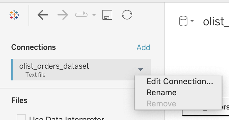
Unzip the archive into a folder. Then open the .twbx file and go to the Data tab in Tableau. You will see the existing data connections pointing to the old file paths. Right-click each data source and choose Edit Connection, then re-point it to the corresponding CSV file in your downloaded folder. This ensures everything works locally on your machine.
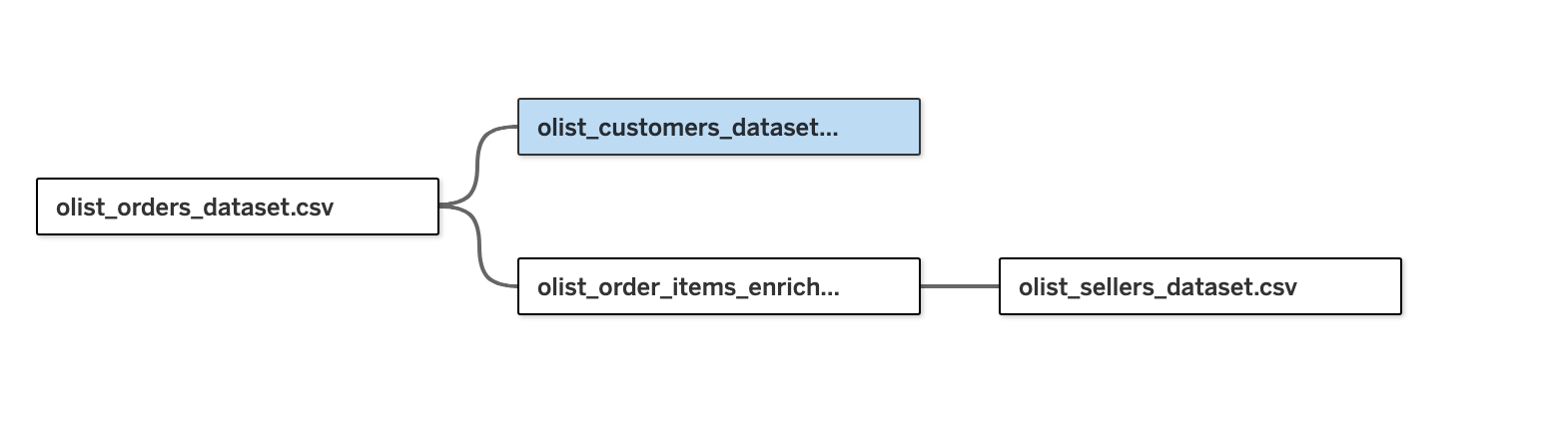
The data model connects these tables:
| Table | Related on | What it adds |
|---|---|---|
| Orders | (base) | Timestamps, status |
| Order Items (enriched) | order_id |
Price, freight, product, English category name (from Syto merge in week 4) |
| Customers | customer_id |
customer_unique_id, state |
| Sellers | seller_id |
Seller location |
A Habit: Test First, Then Visualize
Advanced calculations can surprise you. Before building a chart with a new field, test it in a text table — drag the dimensions and your new field into a simple crosstab, check the numbers, spot-check a few values. Then move to a chart. This removes ambiguity about whether a problem is in the calculation or the visualization.
Session 1: Category Breakdown with Table Calculations
Where we left off
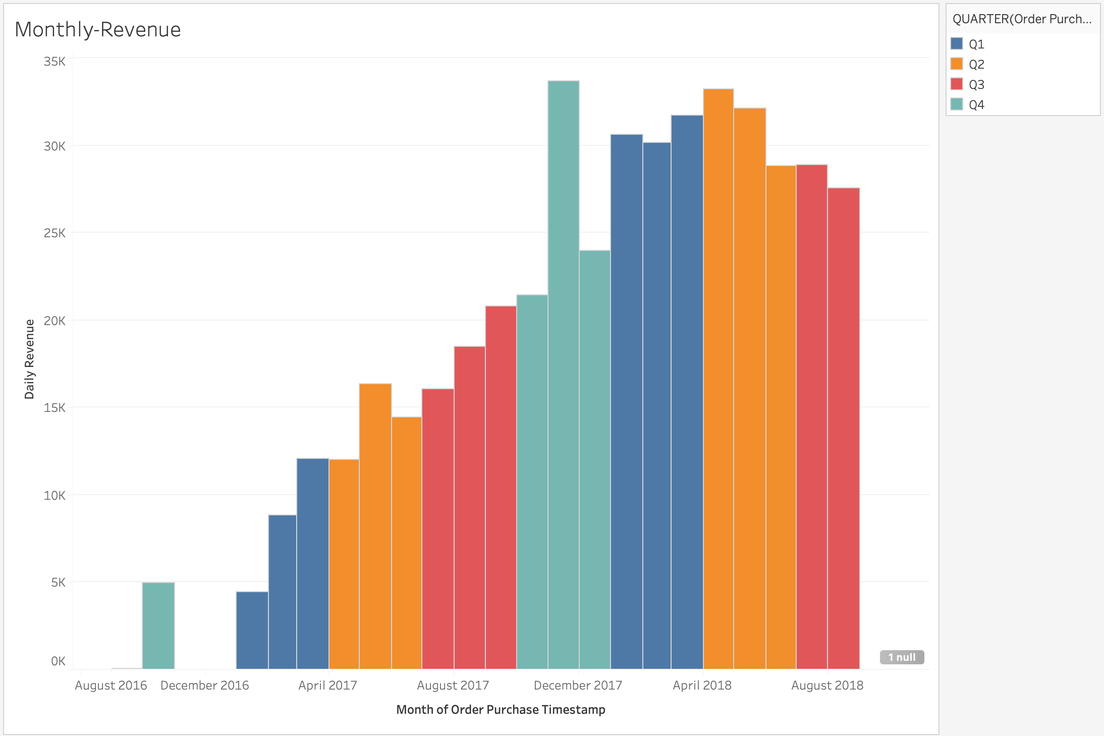
Last week we built a monthly revenue chart colored by quarter. The key finding: Q3 2018 daily revenue is declining, while in the previous year Q3 was still rising. Revenue appears to have plateaued and started dropping. The question is why — which product categories are responsible?
Step 0: Build a Two-Level Category Hierarchy
73 categories are too granular to analyze visually. Use an LLM to create a three-column CSV (product_category_name_english, sub_category, macro_category) with 5-6 macro groups and 15-20 sub-groups.
Before prompting, discuss with your partner: what makes a good prompt here? Consider:
- Should you provide the full list of 73 categories in the prompt, or let the LLM guess?
- What grouping logic makes sense for an e-commerce marketplace — by use case, by buyer type, by product nature?
- How specific should your instructions be about the number of groups?
Review the LLM output critically — does every category land in a sensible group? Then join the CSV to your data on product_category_name_english.
Step 1: Percent Difference of Daily Revenue — Q3 vs Q2 by Category
The goal is a single chart that answers: which macro categories grew or shrank from Q2 to Q3 2018, and how much do they matter?
Build a bar chart where:
- Each bar is a macro category
- Bar length shows the percent difference in average daily revenue between Q3 and Q2 2018
- Bar thickness (size) encodes total revenue contribution of that category — so large categories are visually prominent and small ones are thin
To get there:
- Create a calculated field for average daily revenue (total revenue ÷ number of distinct days in the period)
- Filter to Q2 and Q3 of 2018
- Place macro category on Rows, the percent difference on Columns
- Use Quick Table Calculation → Percent Difference on the revenue measure, computed across Quarter
- Put total revenue on the Size mark to encode category importance
Every table calculation has two settings: what to compute across (addressing) and what to restart on (partitioning). When results look wrong, the first thing to check is the Compute Using direction. Test in a text table first: does each category show one percent-difference value comparing Q3 to Q2?
Step 2: Start a Dashboard
Combine your views into a dashboard layout:
- Monthly revenue chart (from last week) at the top — this is the context
- Category percent-difference bar chart below — this is the drill-down
Add a descriptive title to each view. This is the beginning of a dashboard you will continue building in Session 2.
Optional: Running Total Revenue by Day-of-Quarter
If time allows, build a chart that compares cumulative revenue trajectories across quarters:
- Create a calculated field:
DATEDIFF('day', DATETRUNC('quarter', [Order Purchase Timestamp]), [Order Purchase Timestamp])— this gives you “day 0, day 1, day 2, …” within each quarter - Place this on Columns, and
SUM([Price])on Rows - Add Quick Table Calculation → Running Total on the revenue measure
- Put Quarter on Color to compare trajectories side by side
- Filter to the quarters you want to compare (e.g., Q2 and Q3 of 2017 and 2018)
This view shows whether Q3 2018 started slow or fell off partway through — useful context for your stagnation story. If you build it, consider placing it alongside the monthly revenue chart in your dashboard.
Goal by end of Session 1: You can say “Category X is driving the decline because…” with evidence from the percent-difference chart, and you have the start of a dashboard.
Session 2: LOD Expressions + Dashboard
In Session 1, we created a new dimension externally (macro categories via an LLM) and used it to dissect the Q3 decline. Now we will create new dimensions inside Tableau using LOD expressions — computing per-order and per-customer statistics that become reusable columns.
Step 1: Order Value Tiers
The data has one row per order item, but we want to analyze at the order level. LOD expressions let us compute a value at a different grain than the view.
Create the Order Total field:
{FIXED [Order Id] : SUM([Price])}
This gives every row its full order value, regardless of how many items the order contains.
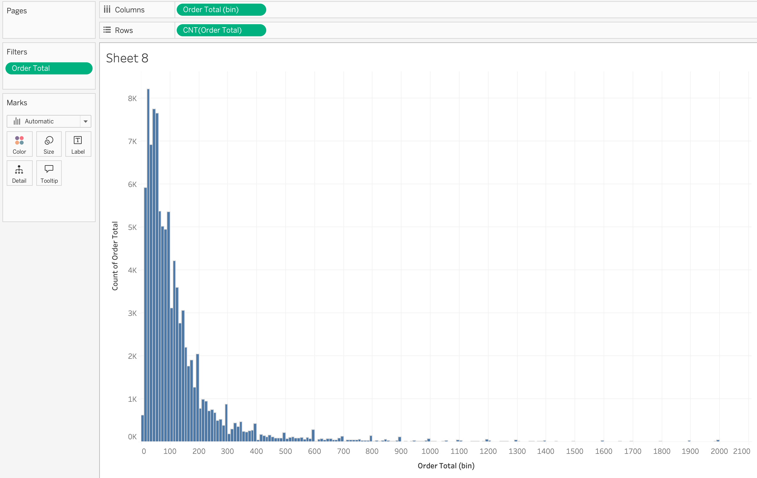
Explore the distribution. Build a histogram of Order Total — you will notice extreme outliers stretching the axis. Filter those out (e.g., exclude values above a reasonable threshold) so you can see where the bulk of orders fall. The ideal bin size is something you should figure out by experimenting — try different values until the shape of the distribution is clear.
Create Order Tiers. Based on the distribution, define three tiers — Small, Medium, and Premium — using an IF/THEN calculated field on Order Total. Choose breakpoints that make sense given where the data concentrates.
Step 2: Percent Difference by Order Tier
Now reuse the same percent-difference chart from Session 1, but replace the macro category dimension with Order Tier. This is the power of having built a reusable chart structure — swap in a different dimension and you get a new angle on the same question.
The chart should show: which order tier (Small / Medium / Premium) declined the most from Q2 to Q3 2018?
Takeaway so far: In Session 1 we found which product categories drove the decline. Now we know which order sizes were affected. Together, these two views pinpoint where the Q3 problem lives — not enough to explain why it happened, but enough to narrow the search.
Optional: Orders per Customer
If time allows, explore repeat-purchase behavior:
{FIXED [Customer Unique Id] : COUNTD([Order Id])}
Note that Customer Unique Id is the true customer identifier (not Customer Id, which can differ across orders).
Build a bar chart of this field. You will find that the vast majority of customers made exactly one purchase — repeat buyers are rare. This means customer-level segmentation would not add much explanatory power here, so it is not worth pursuing further for this analysis. But the LOD technique itself is the lesson.
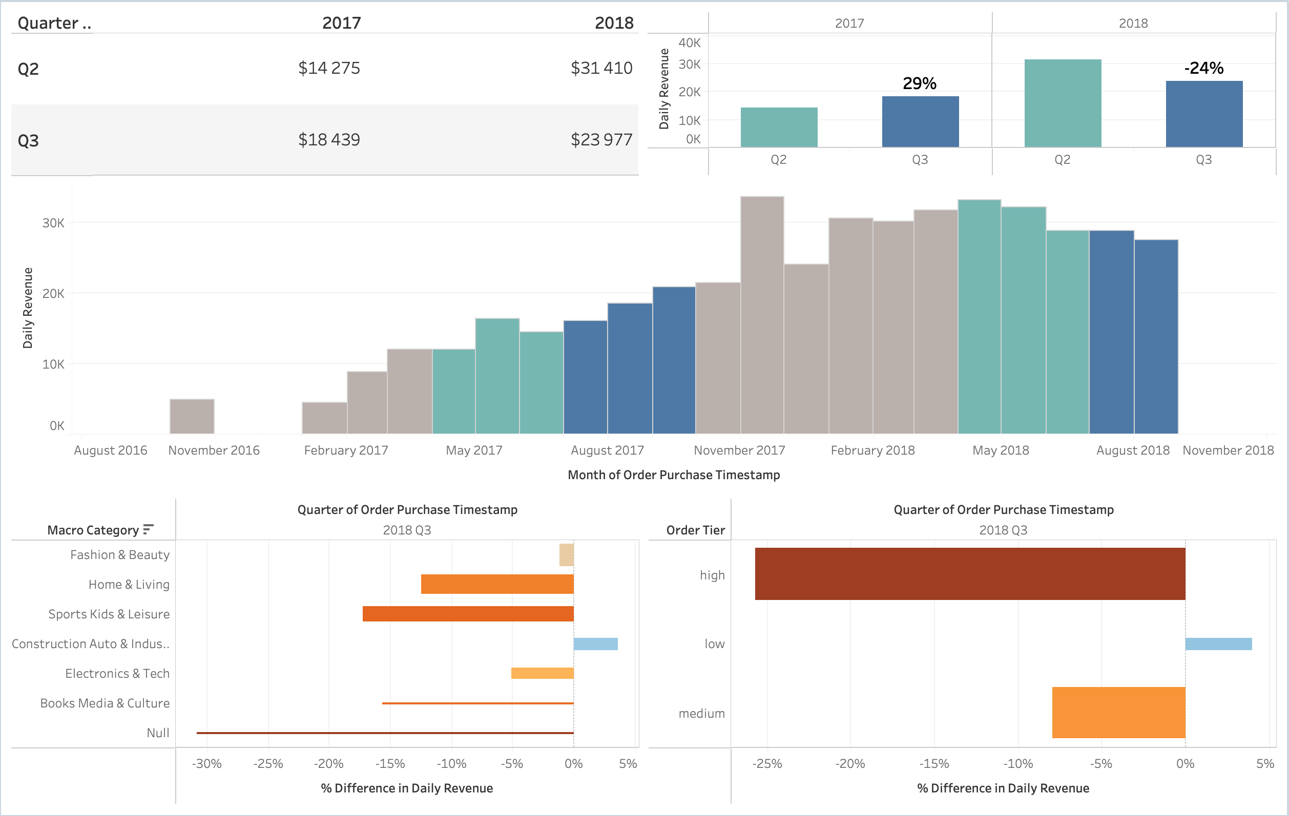
Step 3: Scorecard — Daily Revenue by Quarter
Build a pivot table (text table) showing average daily revenue for Q2 and Q3 in both 2017 and 2018:
- Columns: Year (filtered to 2017, 2018)
- Rows: Quarter (filtered to Q2, Q3)
- Values: Daily Revenue (the calculated field from Session 1)
This gives four numbers that summarize the story: in 2017, daily revenue grew from Q2 to Q3; in 2018, it declined.
Grouped bar chart. Next to the scorecard, build a bar chart with the same data — Quarter on the X axis, grouped by Year, Daily Revenue on Y. Add the percent difference as a label on the Q3 bars so the contrast is visible at a glance (+29% in 2017, -24% in 2018).
Step 4: Assemble the Dashboard
Arrange all views into a single dashboard with three rows:
| Row | Content |
|---|---|
| Top | Scorecard (pivot table) + Grouped bar chart with percent-difference labels |
| Middle | Monthly revenue time series (the original chart from last week) |
| Bottom | Two percent-difference bar charts side by side — one by Macro Category, one by Order Tier |
Polish:
- Titles — descriptive (e.g., “Q3 vs Q2 Daily Revenue Change by Category”), not “Sheet 1”
- Tooltips — 3-4 relevant fields, not the default dump
- Number formatting — currency with thousand separators, percentages where appropriate
- Filter — add at least one filter that applies to all views (Quarter of Order Purchase Timestamp is a good candidate)
Takeaways
- Table calculations run on aggregated results (percent difference, running total, rank). Always check the Compute Using direction.
- LOD expressions compute at a grain you specify (
{FIXED [Order Id] : SUM([Price])}), regardless of the view. They let you create dimensions that don’t exist in the raw data — order tiers, customer segments, etc. - Reusable chart structures save time: swap in a different dimension (macro category → order tier) and you get a new analytical angle without rebuilding the chart.
- Percent difference is a powerful way to compare periods — but the chart needs to also encode magnitude so you know which segments actually matter.
- Test first in a text table, then visualize.
- A dashboard tells a layered story: summary numbers at the top, trend in the middle, drill-downs at the bottom.