Week 1 Practice: Spreadsheet Fundamentals
BUS220 - Business Intelligence and Analytics
Submission Checklist
2 points (satisfactory completion) | Deadline: 3 days after the practice session
Submit a link to your Google Sheet in Moodle. Before submitting, make sure:
Learning Objectives
- Understand how spreadsheets store data internally vs how they display it (data types, formatting, locale)
- Create derived columns using date functions, arithmetic, and conditional logic
- Use lookup functions (XLOOKUP, VLOOKUP) to combine data from multiple sheets
- Build basic pivot tables to summarize data by categories
- Identify when aggregation methods matter (count, sum, unique count)
Tools & Files You’ll Need
- Google Sheets (use your KSE Google account)
- Dataset: Superstore Orders — open the shared spreadsheet
The spreadsheet contains three sheets:
| Sheet | Contents |
|---|---|
| Orders | ~10,000 rows of e-commerce transactions (order dates, products, sales, profit, shipping info) |
| Returns | List of returned order IDs |
| People | Regional manager assignments by region |
Before You Start
- Open the shared spreadsheet link above
- Go to File → Make a Copy and rename it:
BUS220 - Week 1 - <Your Name> - Tick “Share it with the same people”
- Set up your locale (see next section)
Locale Setup
Locales control how numbers and dates are displayed. Since the course materials use US English formatting, we need everyone on the same setting.
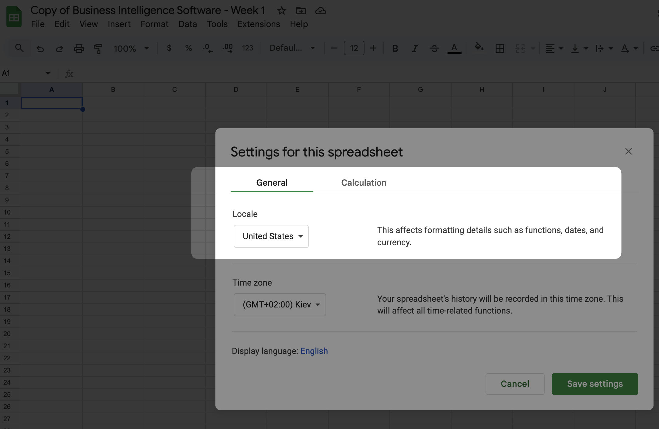
Go to File → Settings, then change the Locale to United States.
In Ukrainian locale, the number one thousand two hundred thirty-four and fifty-six hundredths is written as 1 234,56 — with a space as thousands separator and comma as decimal separator. In US locale, the same number is 1,234.56. The underlying value is identical — only the representation changes. This is your first example of a theme we’ll return to throughout today’s session: what you see is not always what is stored.
Check that it worked:
- In an empty cell, type
=DATE(2020, 5, 18). You should see5/18/2020. - In two other cells, type
123.45and234.56. Add them together — the result should be358.01.
If the date shows as 18/05/2020 or the numbers don’t add correctly, your locale isn’t set to United States yet.
Practice Session 1: Data Types & Derived Columns
Imagine you’ve just joined a company as an analyst. Your manager hands you a spreadsheet of sales transactions and says: “We need to understand how the business is performing — by region, over time, and by product category. Can you prepare the data so we can build a dashboard next week?”
That’s what we’ll do today. The raw dataset has transactions, but not the derived metrics (margins, durations, flags) or the summaries (totals by region and year) that make it useful for decision-making. By the end of both sessions, you’ll have enriched the data and built your first summary views.
Part 0: Explore the Data
Before writing any formulas, take a few minutes to understand what you’re working with. Open the Orders sheet and look at the first 20-30 rows.
Try to answer these questions:
- What does each row represent? Is it one order? One customer? One product? Look at the Order ID column — do you see the same Order ID in multiple rows? What differs between those rows?
- How many rows and columns does the dataset have? (Hint:
Ctrl+Endjumps to the last cell with data.) - What types of information are in the columns? Which columns look like dates, which are numbers, which are text? Are there any columns where the type is ambiguous?
- Look at the other two sheets (People and Returns). How many rows does each have? What column could you use to connect them back to the Orders sheet?
The Orders sheet has ~10,000 rows but only ~5,000 unique orders. Each row is one product line item within an order — a single order with 3 different products appears as 3 rows. This distinction between “row” and “order” will matter every time you count or aggregate.
Part 1: Storage vs Display
Spreadsheets store every value in one of a few internal types: number, text, boolean, or error. Everything you see on screen — dates, currencies, percentages — is just a number with formatting applied on top. When you don’t know this, things break in confusing ways.
Dates are numbers
- Find any cell in the Order Date column (e.g., cell F2)
- Note the date displayed (e.g.,
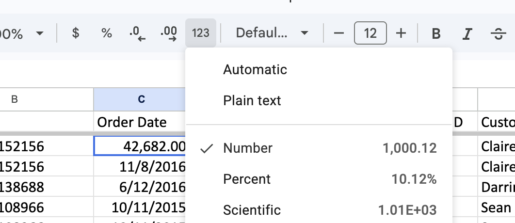
1/3/2014) - Now select that cell and change its format: Format → Number → Number
- You should see a number like
41642— that’s what the spreadsheet actually stores (days since December 30, 1899) - Change the format back to Date
Try this: In an empty cell, enter the formula =F3 - F2 (using two different Order Date cells). The result is a number — the difference in days. This works because dates are numbers underneath.
Try this: In an empty cell, enter =TODAY(). Format it as a number. This is today’s date as a serial number.
Text that looks like numbers
- In an empty cell, type
12.50— this is stored as a number - In the next cell, type
'12.50(with an apostrophe at the start) — this is stored as text - They look the same on screen. Now try
=SUM()on both cells — only the number is included - Use
=ISNUMBER(cell)on each to confirm: one returns TRUE, the other FALSE
If data is imported from a CSV or another system, numeric columns sometimes arrive as text. Functions like SUM, AVERAGE, and VLOOKUP will silently skip or fail on text-that-looks-like-numbers. This is the most dangerous type of bug — it doesn’t fail, it just gives you wrong numbers.
Booleans
- In an empty cell, type
TRUE. In the next cell, typeFALSE - Format both as Number — you’ll see
1and0 - This means you can do math with booleans:
=TRUE + TRUEgives2
Number formatting as “costumes”
- In an empty cell, type
0.1525 - Without changing the cell, apply different formats and observe how the display changes while the formula bar always shows
0.1525:
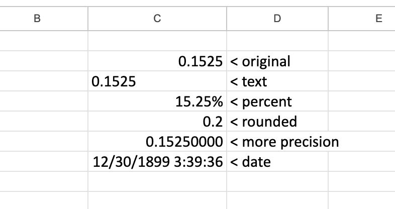
Formatting never changes the stored value. When you format a number as currency, you’re adding a label — not converting it. When you format a number as a percentage, the display multiplies by 100, but the stored value doesn’t change.
Part 2: Cell References — Relative vs Absolute
When you write a formula and fill it down (or across), the cell references shift automatically. This is usually what you want — but not always.
Build a simple pricing model
- In a new sheet (or an empty area), create this small table. You can copy the data below and paste it into cell A1, then use Data → Split text to columns (with comma as separator):
Product,Price,With Tax
Widget,100,
Gadget,250,
Gizmo,75,
,,
Tax Rate,20%,- In cell C2, enter:
=B2 * (1 + B6) - This should give you
120(100 × 1.20). Looks correct. - Now fill down from C2 to C4.
What happened? C3 and C4 probably show wrong values or 0. Look at the formula in C3 — it shifted to =B3 * (1 + B7). The reference to B6 (your tax rate) moved to B7, which is empty.
Fix it with absolute references
The $ sign locks a reference so it doesn’t shift when you fill:
B6— both column and row shift (fully relative)$B$6— neither shifts (fully absolute)B$6— column shifts, row is locked$B6— column is locked, row shifts
- Change the formula in C2 to:
=B2 * (1 + $B$6) - Fill down again. Now all three products calculate correctly using the same tax rate.
- Change the tax rate in B6 to
25%— all three prices update instantly. This is the power of absolute references: one cell controls the calculation for the entire column.
If a formula references data in the same row (like a price on the same row), use relative references — you want them to shift. If a formula references a fixed value (like a tax rate, exchange rate, or lookup range), use absolute references.
You’ll use absolute references again in Session 2 when writing XLOOKUP formulas — the lookup ranges must be fixed, while the search value should shift row by row.
Part 3: Creating Derived Columns — Dates
Useful information is often not stored directly but can be derived from existing columns. Dates are a good starting point.
Go to the Orders sheet. You’ll create new columns at the end of the dataset (or insert them near relevant columns if you prefer to keep things organized).
Year and Month
Create two new columns with headers Order Year and Order Month.
Use these functions (assuming Order Date is in column F):
=YEAR(F2)
=MONTH(F2)
Fill down for all rows. These functions extract the year and month components from the date’s serial number.
Quarter (optional challenge)
There’s no single QUARTER function in Google Sheets. You’ll need to derive it from the month number.
Hint: Months 1-3 → Q1, months 4-6 → Q2, months 7-9 → Q3, months 10-12 → Q4. Think about what arithmetic operation maps these groups to 1, 2, 3, 4.
Shipment Duration
Create a column Shipment Duration that calculates the number of days between the ship date and order date:
=G2 - F2(Adjust column letters to match your sheet — G should be Ship Date, F should be Order Date.)
Most values should be between 0 and 7.
Part 4: Creating Derived Columns — Arithmetic
Now create columns from the numeric fields. These are common metrics you’d compute in any sales dataset:
Cost
The dataset has Sales and Profit, but not Cost. Think about the relationship: Profit = Sales − Cost. Rearrange to derive Cost.
Sales per Item
How much revenue does one unit generate in a given order? You have Sales and Quantity columns.
Profit Margin
What fraction of each sale is profit? Express it as a ratio of Profit to Sales, then format the column as Percent.
Most margins should be between -50% and 50%. You will see some extreme outliers (down to -275%) — these come from rows with very high discounts (80%), where the selling price drops far below cost. That’s not a bug in your formula.
If you see values like 0.12 without the percent sign, the number is correct — just apply percentage format.
Part 5: Creating Derived Columns — Conditional Logic
Is Profitable
Create a column that returns TRUE if the order made money (Profit > 0) and FALSE otherwise.
Remember from Part 1 — TRUE/FALSE are stored as 1/0 internally, so you can sum them later to count profitable rows.
Is Discount
Create a column that flags whether a discount was applied to the order. Check whether the Discount column is non-zero.
At this point, your Orders sheet should have 7-9 new columns. Take a moment to scroll through and verify that the values make sense.
Practice Session 2: Lookups & Pivot Tables
In Session 1, you enriched the Orders sheet with derived columns — dates, metrics, and flags. But all that data is still at the level of individual line items: 10,000 rows that no one can read top-to-bottom.
In this session, you’ll first connect the Orders sheet to the other two sheets (People and Returns) using lookup functions. Then you’ll learn pivot tables — the tool that turns thousands of rows into compact summaries a manager can actually read. This is the core of business intelligence: aggregate and summarize raw data into something that supports decisions.
Part 1: XLOOKUP — Regional Managers
The People sheet has two columns: the regional manager’s name and the region they manage. We want to add this information to every row in the Orders sheet.
This is a lookup operation — for each order, find its region in the People sheet and return the corresponding manager name.
Using XLOOKUP
Create a new column in Orders called Regional Manager. Your goal: for each order, look up its Region in the People sheet and return the corresponding manager name.
Look up the XLOOKUP function in Google Sheets. It takes three arguments:
- Search value — what to look for (the region of this order)
- Lookup range — where to search (the Region column in the People sheet)
- Result range — where to get the answer (the Person column in the People sheet)
Remember from Part 2: the lookup ranges reference the People sheet and should not shift when you fill down. Use absolute references ($) for the ranges, but keep the search value relative so it moves row by row.
Fill down for all rows.
Check your result: You should see one of four manager names (Anna Andreadi, Chuck Magee, Kelly Williams, or Cassandra Brandow). If you see #N/A errors, check that your region column reference is correct.
Using VLOOKUP (alternative)
VLOOKUP is an older function you’ll encounter in existing spreadsheets. Try to achieve the same result using VLOOKUP instead.
Look it up — it works differently from XLOOKUP. Pay attention to:
- The range must start with the search column (not the result column)
- You specify which column to return by number (e.g., 2nd column)
- The last argument should be
FALSEfor exact match
Key limitation of VLOOKUP: It can only search in the leftmost column of the range and return values to the right. If the People sheet had the columns in reverse order (Name first, Region second), VLOOKUP couldn’t look up by Region. XLOOKUP doesn’t have this limitation.
You don’t need both columns — pick one approach. The point is to understand that both exist and when each is useful.
Part 2: COUNTIF Across Sheets — Returned Orders
The Returns sheet lists order IDs that were returned. We want to flag each order in the Orders sheet as returned or not.
This is different from the lookup above — we’re not retrieving a value, we’re checking whether an order exists in another list.
Step 1: Check for existence
Create a column Is Returned. Use the COUNTIF function to count how many times each order’s Order ID appears in the Returns sheet. The result should be 0 (not returned) or 1 (returned).
Hint: COUNTIF takes two arguments — the range to search in, and the value to count. You’ll need to reference the Order ID column in the Returns sheet.
Step 2: Add labels
A 0/1 column works, but text labels are easier to read in pivot tables. Wrap your COUNTIF in an IF to produce “Returned” or “Not Returned” labels instead.
Fill down for all rows.
The Orders sheet has one row per product within an order, but the Returns sheet has one row per order. So all products within a returned order will be flagged as “Returned.” In real life, partial returns are possible — but for this dataset, returns apply to the entire order.
Check your result: Most orders should show “Not Returned.” If everything shows “Returned” or everything shows “Not Returned,” check that you’re referencing the correct Order ID columns in both sheets.
Part 3: Pivot Tables — Basics
Pivot tables summarize rows into a compact table by grouping and aggregating — the same idea as GROUP BY in SQL or .groupby() in pandas.
Create your first pivot table
- Click on any cell in the Orders data (e.g., A1)
- Go to Insert → Pivot Table
- Select New Sheet and click Create
You’ll see an empty pivot table editor on the right side of the screen:
![]()
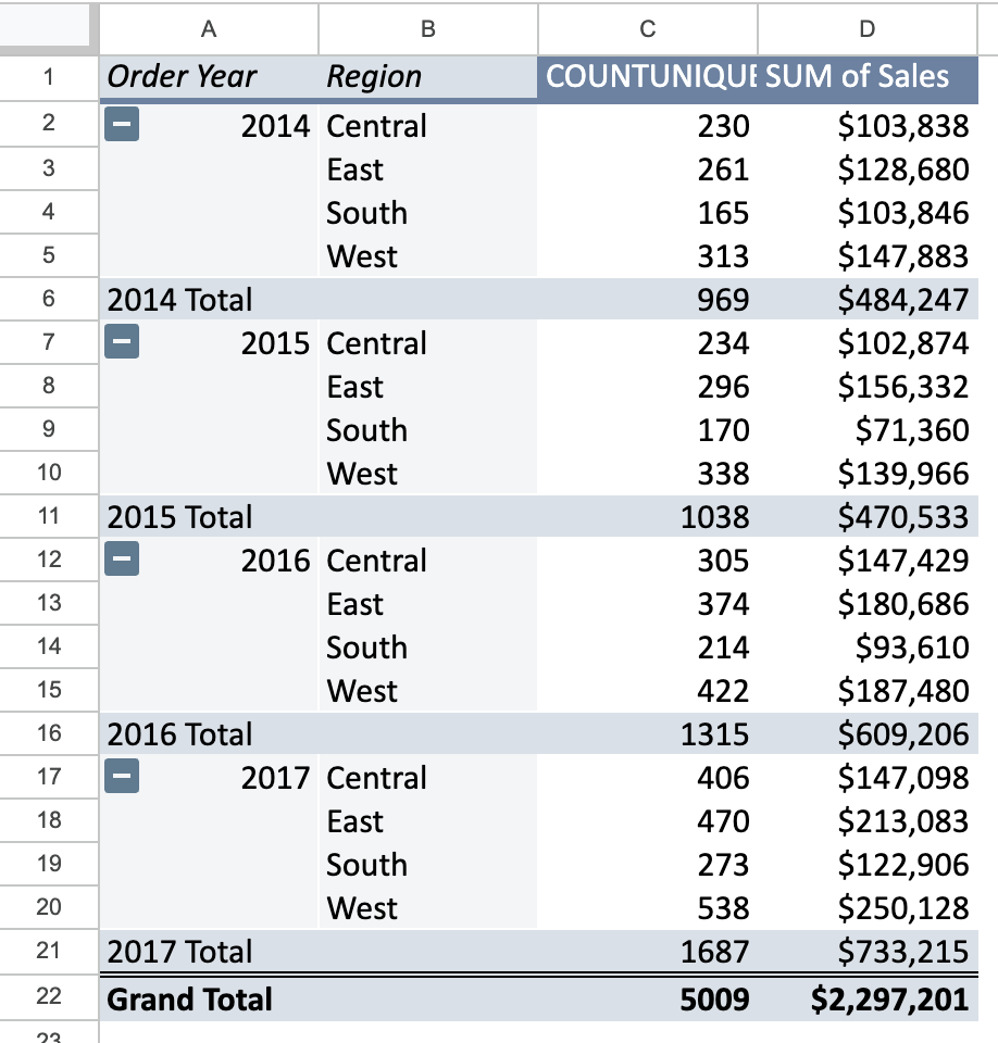
Build a Region × Year summary
Configure the pivot table:
- Rows: Region
- Columns: Order Year (the derived column you created in Session 1)
- Values: Order ID, summarized by COUNTUNIQUE
Your result should look like this:
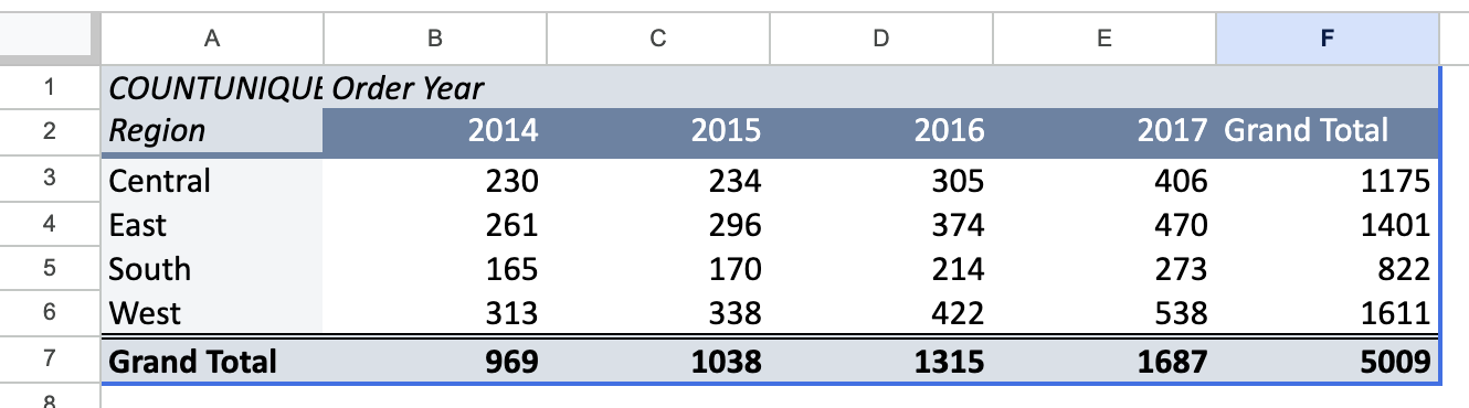
Check your result: The Grand Total should show 5009. If you see ~10,000 instead, you’re using COUNT (which counts rows) instead of COUNTUNIQUE (which counts distinct orders).
Add a second metric
Now add another value: Sales, summarized by SUM.
You’ll notice the table gets wider. Switch “Show as” (sometimes called “Values layout”) to Rows — this stacks the two metrics vertically under each region instead of side by side.
Experiment with layout: Try moving the Year field from Columns to Rows (above Region). Switch “Show as” back to Columns. This layout is often cleaner when you have multiple metrics — each metric gets its own column, and the rows show Year → Region hierarchy.
Read the pivot table
Now step back from the mechanics and look at what the numbers tell you:
- Which region has the most orders? Is it also the region with the highest total sales? If not, what might explain the difference?
- Is the business growing? Compare 2014 totals to 2017 totals. Is the growth even across regions, or are some regions growing faster?
- What’s the average order value (total Sales ÷ unique Orders) per region? You can calculate this outside the pivot table or mentally estimate it. Does any region stand out?
You couldn’t answer these by scrolling through 10,000 rows. The pivot table made the same data readable in 30 seconds.
Part 4: Pivot Tables — Calculated Fields
Pivot tables can also create their own calculations. This matters because some metrics break if you summarize a pre-calculated column.
The weighted average problem
Consider this example:
| Product | Sales | Profit | Profit Margin |
|---|---|---|---|
| A | $100 | $10 | 10% |
| B | $990 | $495 | 50% |
If you average the Profit Margin column: (10% + 50%) / 2 = 30%
But the correct overall margin is: $505 / $1,090 = 46.3%
The naive average treats both products equally, ignoring that Product B has 10× the sales volume. The correct approach is to divide the total profit by total sales.
See it in your pivot table
- Add the Profit Margin column (from Part 3 of Session 1) to your pivot table values
- Set it to AVERAGE — this is the naive approach
- Now add a Calculated Field: click the “Calculated Fields” section in the pivot editor. Create a field that computes the correct weighted margin — divide the sum of Profit by the sum of Sales.
- Compare the two columns. They won’t match — the calculated field gives the correct weighted result. Look at the Central region in particular: the naive average shows a negative margin, while the correct weighted margin is positive. The naive average is dragged down by a few small orders with extreme discounts, even though the region is profitable overall.
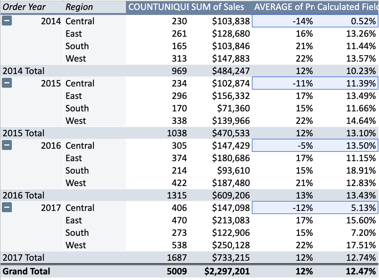
If you divide the SUM of Profit by the SUM of Sales from your pivot table, you’ll confirm that the calculated field is correct.
When aggregating ratios (margin, rate, percentage), always compute them from aggregated components (sum of profit / sum of sales), not by averaging pre-calculated ratios. You’ll see this again in Tableau.
Bonus Tasks (if time allows)
More pivot tables: Create a pivot table showing Sales and Profit by Category and Sub-Category. Which sub-category has the highest profit margin (using a calculated field)?
Quarter column via pivot grouping: Instead of creating a Quarter column manually, right-click a date in a pivot table and explore Create pivot date group → Quarter. How does this compare to the formula approach?
UNIQUE and FILTER functions: In a new sheet, use
=UNIQUE(Orders!M2:M)to get a list of all regions. Then use=FILTER(Orders!R2:R, Orders!M2:M = "East")to get all sales for the East region. These are modern array functions that are powerful alternatives to pivot tables for quick analysis.Investigate returns by region: Build a pivot table with Year and Region as rows, Is Returned as columns, and COUNTUNIQUE of Order ID as values. Add a formula outside the pivot to calculate the return rate (% of orders returned) per region per year. Which region has the highest return rate?
Common Issues & Troubleshooting
| Problem | Likely Cause | Solution |
|---|---|---|
| Dates show as numbers (e.g., 41642) | Column formatted as Number | Select column → Format → Date |
| SUM returns 0 on a column that has values | Values are stored as text, not numbers | Check with ISNUMBER(). Re-enter values or use VALUE() to convert |
| XLOOKUP returns #N/A | Region value doesn’t match exactly (extra spaces, different case) | Use TRIM() and check for leading/trailing spaces |
| Pivot table shows COUNT instead of COUNTUNIQUE | Wrong aggregation selected | Click the value field in pivot editor → change “Summarize by” to COUNTUNIQUE |
| Fill-down changes lookup ranges | Missing $ in absolute references | Use $ signs: People!$A$2:$B$5 |
| Locale issues — decimal comma instead of point | Locale not set to US | File → Settings → Locale → United States |
| VLOOKUP returns wrong value | Column index is off because you inserted columns | Recount the column position in the range, or switch to XLOOKUP |
Key Takeaways
- Storage vs display: Dates are numbers, booleans are 0/1, formatting is a costume. What you see is not always what is stored.
- Locale matters: The same value looks different in different locales. When collaborating, agree on a locale to avoid confusion.
- Relative vs absolute references: Use
$to lock references that should stay fixed when filling down (tax rates, lookup ranges). If fill-down gives wrong results, this is the first thing to check. - Derived columns let you extract information that’s implicit in the data (year from date, margin from sales and profit).
- IF creates categories from continuous data — turning numeric thresholds into yes/no flags.
- Lookups connect data across sheets. XLOOKUP is more flexible; VLOOKUP is more common in older spreadsheets.
- COUNTIF across sheets checks for existence — useful when one table is a subset of another (returns, flags).
- Pivot tables summarize data by categories. Always use COUNTUNIQUE for counting distinct items like orders.
- Never average a ratio. When aggregating percentages or margins, compute from summed components instead.