Week 2 Practice: Charts, Conditional Formatting & Dashboards
BUS220 - Business Intelligence and Analytics
Submission Checklist
2 points (satisfactory completion) | Deadline: 3 days after the practice session
Submit a link to your Google Sheet in Moodle. Before submitting, make sure:
Learning Objectives
- Apply conditional formatting to make patterns visible at a glance (pre-attentive attributes in action)
- Create and customize bar charts, line charts, and stacked area charts in Google Sheets
- Build a pivot table to aggregate data before charting
- Assemble multiple charts into an interactive dashboard with slicers, scorecards, and sparklines
- Structure a spreadsheet so someone else can read and trust it
Tools & Files You’ll Need
- Google Sheets (use your KSE Google account)
- Dataset: Your copy of the Superstore spreadsheet from Week 1
If you don’t have your Week 1 spreadsheet, make a new copy from the shared spreadsheet and re-create the derived columns from last week (Order Year, Shipment Duration, Cost, Profit Margin, Is Profitable, Regional Manager, Is Returned).
Before You Start
- Open your Week 1 spreadsheet
- Duplicate the file: File → Make a Copy, rename it
BUS220 - Week 2 - <Your Name> - Verify your derived columns are in place (Order Year, Profit Margin, Regional Manager, etc.)
Practice Session 1: Conditional Formatting & Basic Charts
Part 1: Conditional Formatting
In the lecture, we talked about pre-attentive attributes — visual features like color and intensity that the brain processes before conscious attention kicks in. Conditional formatting is how you apply those attributes to a spreadsheet. Instead of reading hundreds of numbers one by one, you let color do the scanning for you.
Color scale on Profit Margin
- Select your entire Profit Margin column (click the column header)
- Go to Format → Conditional formatting
- In the panel that opens, change “Format cells if…” to Color scale
- Set the scale:
- Min: red (this marks negative margins — losses)
- Midpoint: white, at value
0 - Max: green (this marks healthy margins)
- Click Done
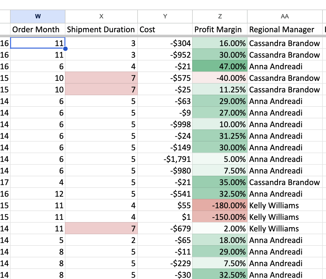
Scroll through the data. You should immediately see which rows are losing money (red) and which are profitable (green) — without reading a single number. That’s the pre-attentive pop-out effect from the lecture.
Check your result: Look at rows with 80% discount — they should be deep red. Rows with 0% discount should be green.
Highlight rule on Shipment Duration
Sometimes color scales are too gradual. For a yes/no question like “did this order ship late?”, a hard threshold works better.
- Select your Shipment Duration column
- Add a conditional formatting rule: Format cells if… → Greater than → 5
- Set the formatting to a red background with bold text
Now you can instantly spot slow shipments across thousands of rows.
Your result should look something like this — profit margins on a red-white-green scale, and late shipments highlighted in red:
Part 2: Structuring Your Spreadsheet for Others
Before we start charting, take a few minutes to make your spreadsheet readable by someone who didn’t build it. In the lecture we talked about audience and purpose — the same principle applies to your data work, not just your visualizations. If a colleague opens your spreadsheet next week, they should be able to understand what’s going on without asking you.
Sheet naming and order
- Rename your sheets so the names describe the content (e.g., “Orders”, “Returns”, “People” — these are probably fine already)
- Check: would a stranger opening this file know which sheet to look at first?
Column header hygiene
- Review your derived columns from Week 1. Do the headers clearly describe what each column contains?
- Rename any ambiguous headers. For example, if you called a column “Margin”, change it to “Profit Margin (%)” — include the unit or format so readers don’t have to guess
Freeze rows and columns
When you scroll through 10,000 rows, the header row disappears. Fix this:
- Click on row 2 (the first data row)
- Go to View → Freeze → 1 row
- Now scroll down — the header stays visible
Also freeze the first few identifier columns (Order ID, dates, customer info) so they stay visible when scrolling right past your derived columns:
- Select the column after the last one you want frozen
- View → Freeze → Up to column [X]
Add a Notes sheet (optional)
Create a sheet called “Notes” or “README” at the beginning of the workbook. Write 3-4 lines: - What dataset this is (Superstore Orders, ~10K transactions, 2014-2017) - What derived columns you added and how they’re calculated - Your name and the date
This takes two minutes and saves anyone who opens the file ten minutes of confusion.
Part 3: Bar Chart — Sales & Profit by Category
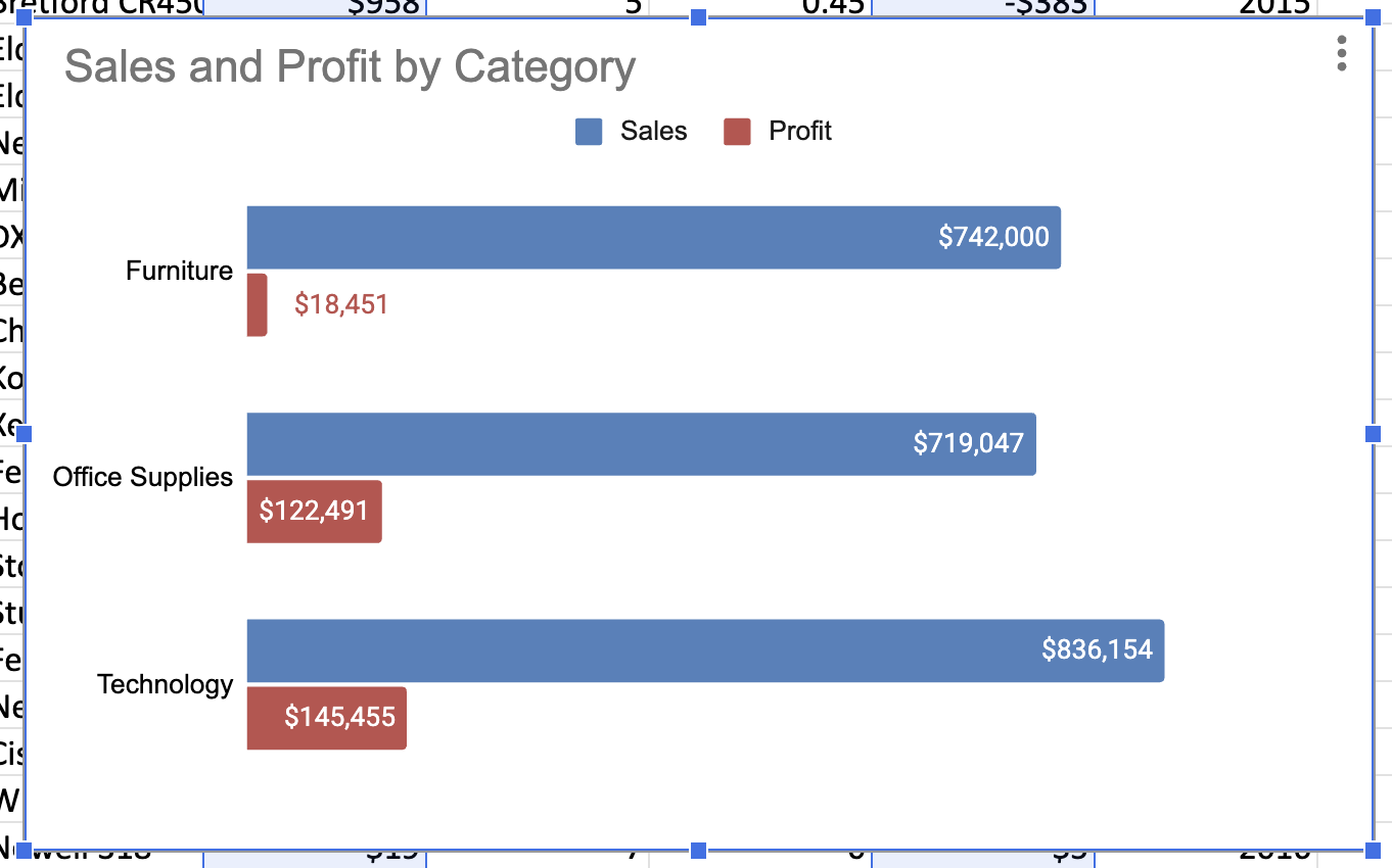
Now let’s apply the chart selection principles from the lecture. Our first question: how do Sales and Profit compare across product categories?
This is a comparison of a few categories on two metrics — a bar chart is the right choice.
Create the chart
- Select the Category, Sales, and Profit columns
- Go to Insert → Chart
- In the Chart editor, select Bar chart as the chart type
- Check the Aggregate checkbox in the Setup tab — this tells Google Sheets to sum values by category automatically
Customize the chart
Explore the Customize tab in the Chart editor. Work through these settings to understand what each one controls:
- Chart style: background color, font, 3D (avoid 3D — remember the lecture)
- Chart & axis titles: add a title “Profits & Sales by Category” and a subtitle “comparison in $ USD”
- Series: enable Data Labels to show values directly on the bars
- Legend: move it to the bottom
- Horizontal axis / Vertical axis: experiment with min/max values, gridlines, label formatting
After you’re satisfied, remove the clutter: turn off gridlines, axis labels you don’t need, and unnecessary formatting. The goal is a clean chart where the data speaks. Try to get something close to this:
Move to its own sheet
Go to the chart’s ⋮ menu → Move to own sheet. Give the sheet a descriptive name like “Chart: Sales by Category”.
Part 4: Line Chart — Quarterly Sales by Region
Our next question: how have sales trended over time across regions?
This is a trend over time with multiple series — a line chart is the right choice (not a bar chart, which would create a cluttered wall of bars).
Why you need a pivot table first
Try selecting Order Date, Region, and Sales columns and inserting a chart directly. Even with Aggregate enabled, you’ll see daily-level data — too granular to read any trends.
Google Sheets charts don’t let you control aggregation granularity. So you need an intermediate step: a pivot table that pre-aggregates to the quarterly level.
Create the pivot table
- Click in the Orders data → Insert → Pivot Table → New Sheet
- Configure it:
- Rows: Order Date
- Columns: Region
- Values: Sales, summarized by SUM
The pivot table initially shows daily dates. To change to quarterly:
- Right-click any date cell in column A → Create pivot date group → Year-Quarter
Your pivot table should now show 16 rows (4 years × 4 quarters) with Sales broken out by region.
Check your result: The 2014-Q1 Central value should be approximately $8,601.
Create the line chart
- Select the entire pivot table (including headers)
- Insert → Chart
- It will likely default to a bar chart — change it to Line chart
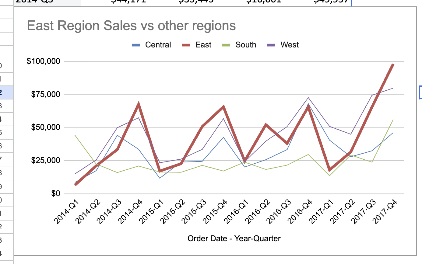
You should see four lines, one per region, tracking quarterly sales from 2014 to 2017.
Focus on one region
With four lines of similar thickness and color, it’s hard to follow any single region’s story. Use the Series customization options to highlight one region:
- Make the East series thicker (line thickness 3-4px) and use a bold color (e.g., dark red with dot markers)
- Make the other three series thinner (1px) and lighter (e.g., gray or light colors)
This creates visual hierarchy — the “East” story pops out while context from other regions stays available.
Give the chart a title like “East Region Sales vs Other Regions” and move it to its own sheet.
Practice Session 2: Dashboard Assembly
In Session 1, you created individual charts. Now you’ll combine them into an interactive dashboard — the kind of view a manager would check regularly to monitor business performance.
Part 1: Stacked Area Chart
Before assembling the dashboard, create one more chart type that shows a different perspective on the same regional sales data.
Stacked area chart
- Go to your quarterly pivot table
- Select the data and insert another chart
- Change the type to Stacked area chart
This shows total sales (the top of the stacked area) and each region’s contribution to it. Notice that you can now see whether total sales are growing, but you lose the ability to track individual regions (except the one at the bottom).
100% stacked area chart
- Duplicate the stacked area chart and change it to 100% stacked area chart
Now the Y axis shows 0-100%, and you can see whether each region’s share of total sales is changing over time. This answers a different question: “Is the East region becoming a larger or smaller part of the business?”
Move both charts to their own sheets.
Reflect: You now have four chart types built from the same quarterly data — line, stacked area, and 100% stacked. Each answers a different question. This is the chart selection principle from the lecture: the data doesn’t dictate the chart — the question does.
Part 2: Assembling the Dashboard
- Create a new sheet called Dashboard
- Go to each chart on its separate sheet, click the ⋮ menu → Copy chart
- Go back to the Dashboard sheet and paste (Ctrl+V)
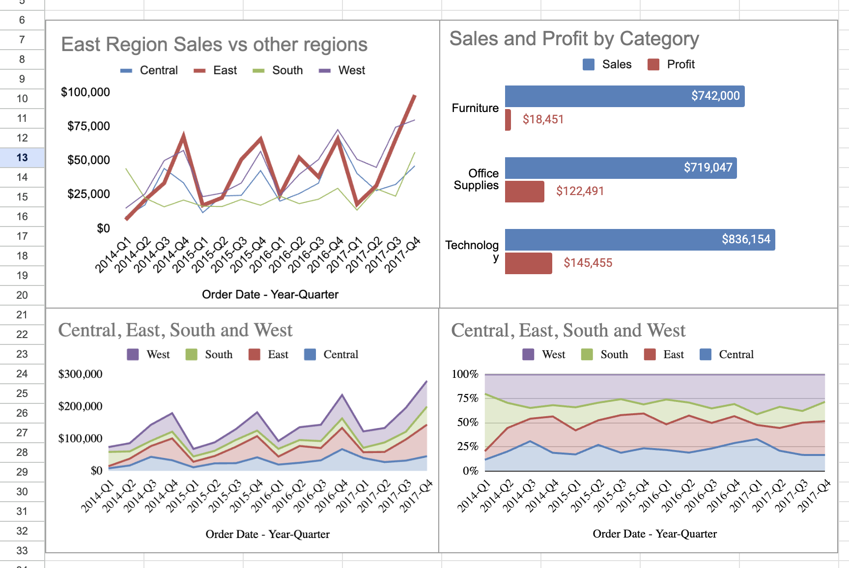
- Arrange the charts in a 2×2 grid:
- Top-left: Line chart (East region focus)
- Top-right: Bar chart (Sales & Profit by Category)
- Bottom-left: Stacked area chart
- Bottom-right: 100% stacked area chart
Resize the charts so they fill the visible area without overlapping. Leave rows 1-7 empty at the top — you’ll use those for slicers and scorecards.
Your dashboard should look something like this at this stage:
Part 3: Adding Slicers
Slicers add interactivity — they let someone filter all charts at once by clicking a button, without editing any data.
- Go to the Orders sheet
- Data → Add a slicer
- Make sure the data range covers the full Orders table
- Set the slicer column to Region
- Copy the slicer and paste it on the Dashboard sheet
Try clicking different regions in the slicer. You’ll notice that only the bar chart reacts to the filter. The line and area charts don’t change — they’re built from pivot tables, and Google Sheets slicers don’t filter pivot table data.
This is a real limitation of Google Sheets as a dashboarding tool. The bar chart works because it’s built directly from the Orders data (with Aggregate), so the slicer filters the underlying rows. But line and area charts need each series in a separate column, which requires a pivot table — and pivot tables sit outside the slicer’s reach.
There’s no clean fix for this in Google Sheets. This is exactly the kind of problem that dedicated BI tools like Tableau solve — filters apply globally to every chart on a dashboard, regardless of how the data is structured. We’ll get there in a few weeks.
For now, your dashboard has partial interactivity: the slicers control the bar chart and scorecards, while the time-series charts show the full unfiltered picture. That’s an acceptable compromise — many real dashboards mix interactive and static elements.
Add two more slicers:
- Segment (Consumer, Corporate, Home Office)
- Category (Furniture, Office Supplies, Technology)
Arrange the slicers in a row across the top of the dashboard.
Part 4: Scorecards & Sparklines
Scorecards
Scorecards are large-format numbers that show key metrics at a glance. In Google Sheets, you create them manually with formulas and cell formatting.
In the Dashboard sheet (below the slicers, above the charts), create cells for:
- Total Sales:
=SUM(Orders!Sales_column) - Total Cost: same approach with your Cost column
- Total Profit: same with Profit column
Like the time-series charts, these totals won’t react to slicers — they always show the overall numbers. Again, this is a Google Sheets limitation that Tableau handles naturally.
Format these cells: - Large font (20-24pt) - Bold - Currency format with no decimals - Add a label above each (“Total Sales”, “Total Cost”, “Total Profit”)
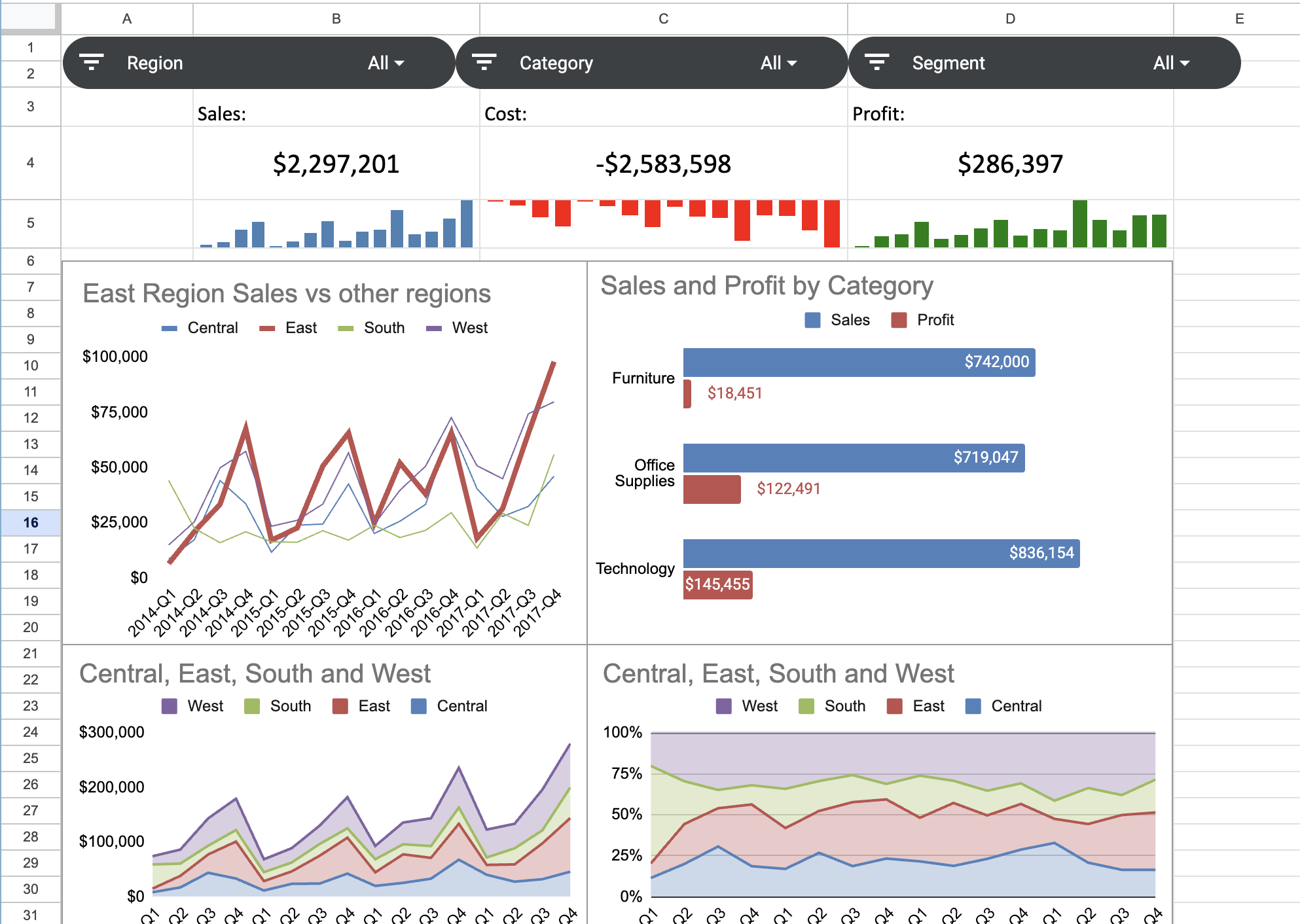
Check your result: With no filters applied, Total Sales should be approximately $2,297,201.
Sparklines
A scorecard shows a single number — but a number alone doesn’t tell you whether things are getting better or worse. Sparklines solve this: they’re tiny charts that fit inside a cell, showing a trend right next to the headline number.
Google Sheets creates sparklines with a formula, not through the chart menu. The SPARKLINE function takes a range of values and renders them as a miniature chart inside the cell.
For this to work, you need quarterly aggregated data. Make sure you have a pivot table (or copied values) on the Dashboard sheet with quarterly Sales, Cost, and Profit totals — the same data you used for the line chart in Session 1.
Below each scorecard, enter the following formula (adjusting the range to point to your quarterly Sales column):
=SPARKLINE(T19:T34, {"charttype", "column"; "color", "steelblue"})The {"charttype", "column"} part tells Google Sheets to draw a column chart. The syntax with curly braces is how you pass options to the SPARKLINE function — each option is a "key", value pair, separated by semicolons.
Use different colors for each metric so they’re easy to distinguish:
- Sales:
"steelblue" - Cost:
"orange" - Profit:
"green"
The sparkline will appear tiny by default — it only fills one cell. To make it bigger, select the sparkline cell plus several cells to the right and click Format → Merge cells. The sparkline will expand to fill the merged area.
Other chart types to try: Replace "column" with "line" for a line sparkline, or "bar" for a single horizontal bar (useful for showing a value relative to a maximum). Experiment to see which reads best for each metric.
Your final dashboard should look something like this — slicers at top, scorecards with sparklines below, and four charts filling the rest:
Bonus Tasks (if time allows)
Average Order Value scorecard: Calculate Sales / COUNTUNIQUE(Order ID) using a pivot table. Add it as a fourth scorecard on the dashboard.
Median Shipment Time scorecard: Use
=MEDIAN()on the Shipment Duration column. Does this metric change interestingly when you filter by region?Conditional formatting on the pivot table: Apply a color scale to the quarterly pivot table values. Which quarter-region combinations stand out as unusually high or low?
Dashboard aesthetics: Align all charts to a grid. Use consistent colors across charts (same color for each region everywhere). Remove unnecessary gridlines and borders. Try to make it look like something you’d present to a manager.
Key Takeaways
- Conditional formatting = pre-attentive attributes applied to a table. Color scales make patterns visible instantly. Threshold-based rules answer yes/no questions.
- Structure your spreadsheet for others — clear headers, frozen rows, and a brief README save everyone time. If a colleague can’t understand your file without asking you, it’s not done yet.
- The question determines the chart, not the data. The same quarterly sales data produced four different chart types, each answering a different question (trend, comparison, composition, share).
- Pivot tables are the bridge between raw data and charts. When you need to control aggregation granularity (daily → quarterly), aggregate first, then chart.
- Slicers make dashboards interactive — but in Google Sheets they only affect charts that reference the filtered data range directly. This is a real limitation you’ll overcome when we move to Tableau.
- Scorecards and sparklines give your dashboard a quick-read layer. A manager should be able to glance at the top of your dashboard and know the headline numbers and trends.